8.5. Rivers

The “River” boundary condition is used to simulate interactions between a routed river and an aquifer. The routed-river function uses Manning’s equation to calculate the flow in an open channel. A given reach of the river is represented by a node and corresponding reach length. Each reach is connected to the next reach by sequencing the nodes from upstream to downstream. River-groundwater system interactions are simulated by comparing the head in the groundwater system to the head in the river over time and by transferring water across the riverbed accordingly. Rivers can be connected to form a river network. External sources of water to rivers are termed “tributaries.”

The physical accuracy of a river’s representation depends upon the number of nodes used to resolve the geometry of the river in plan view and the physical coefficients used to calculate gains and losses to and from the river.

When “River” is selected from the “BCs” drop-down menu on the Main Menu banner at the top of the screen, the dialog box shown in appears.

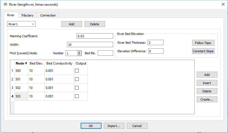
Figure 8.12 The “River” tab of the “River” dialog box

Rivers are defined by clicking the “Add” button at the top of the “River” tab of the “River” dialog box. Unlike boundary conditions such as pumping wells, constant heads, drains, or variable-flux boundaries, rivers cannot be created using any plot items. A river can only be created in the following two ways:

1. From a “BLN” File: This is done by clicking the “Create” button on the lower right of the “River” tab, which opens the “Select BLN file” dialog box. After selecting the appropriate .BLN file, click “Open” and MINEDW automatically selects the appropriate nodes based on distance from the .BLN defined line. MINEDW then calculates the riverbed elevations and the elevation difference between the upstream and downstream node.

2. Manually: The user can manually enter node numbers; riverbed elevations can then be automatically generated by MINEDW using the “Follow Topo” button.

For any river, the user has the choice of calculating the slope based off the topography using “Follow Topo,” which is the default setting, or applying a “Constant Slope.” For the “Constant Slope” option for the entire river channel, the “Slope” box will become active and the “Bed Elev.” column of the table will no longer be visible. The slope of all segments of the river will be constant. If the “Constant Slope” option is used, then the “First (Lowest) Node Bed Elevation” is used as a reference to calculate other bed elevations. When using “Constant Slope,” if the river is connected to another river, the elevation of the node that forms the river connection is used as the reference elevation rather than the “First (Lowest) Node” and “Bed Elev.”

For each river, the “Manning Coefficient.” river channel “Width,” “First (Lowest) Node,” “Bed Elev.,” and bed hydraulic conductivity must be defined. The following is an explanation of the required information:

• Manning’s Coefficient: Empirical coefficient for river depth [TL^-1/3].

• Width: Coefficient for river width [L].

• First (Lowest) Node: The node number of the lowest node, which should correspond to the first node forming the river.

• Bed Elev.: The elevation of the riverbed at the downstream node forming the river [L].

Additionally, for each node composing the river, the following must be defined:

• Node: The node number for nodes forming the river.

• Riverbed elevation: The elevation of the riverbed at the node (optional if “Constant Slope” is used) [L].

• Bed Conductivity: The riverbed hydraulic conductivity [LT^-1].

• Output: Option to print simulation results for the node to the output file. At a minimum the results at the end node, or any connected node, will be printed out.

Next, “Tributaries” are entered. “Tributaries” are inflows of water to the river and can be used to simulate inflow from outside the model domain or discharge from an outfall such as a lined channel, pump, etc. inside of the model domain. The flow from a tributary can be “Constant,” “Annual,” or “Varied.” shows the “Tributary” tab of the “River” dialog box.

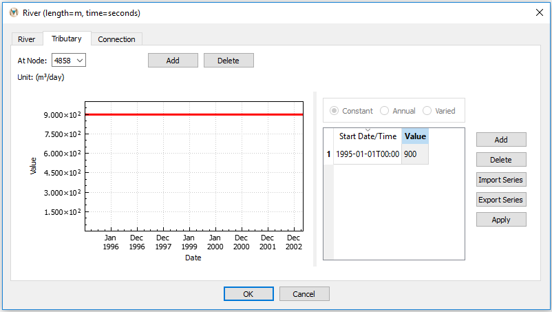
Figure 8.13 The “Tributary” tab of the “River” dialog box

Tributaries are added by clicking the “Add” button at the top of the window and specifying the node at which the inflow occurs. The start date of the inflow and the amount of inflow in m³/day or cubic feet per day (ft³/day) can be specified in the time-series table on the lower right. The graph to the left of the table shows the inflow values over time. A time series may be imported as a .DAT file using the “Import Series” button.

The last tab in the “River” dialog box, shown in Figure 8.14, describes the connections between individual rivers and between rivers and tributaries. The user does not need to specify the connection points but can check here to ensure that the rivers and tributaries are connected correctly. If any changes to the river network have been made or a new river network has been created, clicking the “Refresh” button redefines the connections.

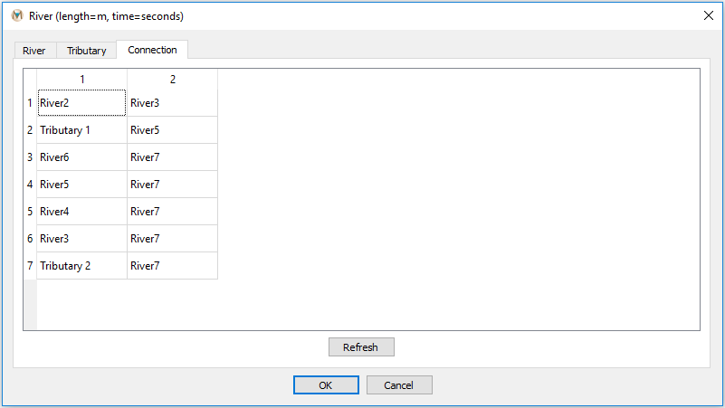
Figure 8.14 The “Connection” tab of the “River” dialog box