Three-Dimensional Vibrations
The project file for this example may be viewed/run in FLAC3D.[1] The main data file used is shown at the end of this example.
Problem Statement
This example shows how FLAC3D can be used to predict blast induced vibrations at a mine scale when features like geological layering and subsurface excavations are present. In typical engineering practice, the scaled-distance approach is used to predict vibrations for a problem like this. The scaled distance analysis has the limitations that the explosive is represented as a point source, the rock is taken as homogeneous, and the wave path is treated as a straight line. This example demonstrates that a numerical analysis of blast induced vibrations can overcome limitations and provide good insights into how vibrations and damage are distributed around a blast.
The file geometry.py creates a set of three 10 m high benches in a model that is 18.5 m wide. Two rows of two blastholes are placed with 6 m spacing and 4 m of burden to the free face. Each hole is 11m deep, accounting for 1 m subdrill, and each hole has 4 m of stemming. The blastholes are conceptually 200 mm diameter and the model resolution is 0.5 m, so the blast holes are larger than the conceptual blastholes. As discussed below, this is accounted for by applying the known blast inducted stress history from the 1D explosive rock example in each hole. Two 5 m by 4 m by 5 m stopes are excavated below the middle bench and the bench is composed of three rock types. The bottom of the blastholes is taken as the reference depth of 0. From the bottom of the model to a height of 8 m, the strongest rock is present with a density of 2,650 kg/m3 and a Young’s modulus of 35 GPa; above a model height of 8 m but below 17 m the rock has 10% lower density and a Young’s Modulus of 3.5 GPa; above 17 m the rock has a Young’s modulus of 1.75 GPa. The model has no gravity and all initial stresses are zero. The model boundaries at free surfaces have the energy absorbing quiet boundary condition applied to prevent stress wave reflections at these boundaries.
Relative to 1D explosive rock example and the Programmed burn example examples, a simplified approach is taken in this example that focuses on elastic wave propagation. A mine-scale mesh represents a section of an open pit with a mesh of elements around 0.5 m in size. Relative to 1D explosive rock example, this model has large elements and uses an elastic constitutive behavior. The blast-induced stress wave predicted by the 1D model is recorded at a radial distance of 25 cm (half the grid resolution) and is applied to this model as a time-varying applied pressure boundary condition inside each blasthole. The \(xx\) component of stress history in the 1D model is shown in Stress at 25 cm. This plot shows some high frequency oscillations and has more details than are needed for this model. The applied pressure wave form is simplified as a triangle wave with a rise time of 0.1 ms, a peak pressure of 800 MPa, and a decay time of 1.5 ms.
There is an implicit assumption in this coupling procedure that wave energy in high frequencies (that cannot be represented in the coarse model due to the Nyquist limit) is attenuated and is not relevant to rock damage. Given the grid size and elastic properties, frequencies around a thousand Hertz can be represented, well above the 10 to 300 Hz frequency range that cause the most rock damage.
A diagonal timing pattern with 5 ms interhole delay and a velocity of detonation of 4600 m/s are used to off set the pressure pulse for zone faces in each hole and at each height along the explosive charge. The cmd:\(zone.face.apply\) command is used to set a different time-varying pressure boundary condition for each face representing the explosive charge. Most decrease in PPV with distance from the charge is due to geometric effect, but a small amount of stiffness proportional Rayleigh damping is used to represent inelastic attenuation.
Results
The model is run in dynamic mode two in stages: first to around 2 ms where the first hole to detonate is nearly complete, and onwards to about 25 ms when the majority of the dynamic effects are over. Model results are shown on a cut away plan that intersects the first row of blastholes and one of the stopes. Peak particle velocity (PPV) is tracked during the calculation. Figure Figure 3 shows the instantaneous gridpoint velocity magnitude; the Mach cone can be seen.
The remaining figures show the model at the end time of 25 ms. Gridpoint PPV at the end of the model time. shows the PPV induced by the blast and Gridpoint PPV on the stopes. shows the PPV on the stopes. Note that the color scale limits are different in each image. The model shows that there is some internal reflection at the lithological boundary at \(z\) = 8 m, there is a surface amplification effect at the bench tops and faces, and that there is an amplification around the stopes due to reflection and channeling of wave energy into the pillars.
This type of analysis is typically done empirically with the scaled distance formula so it is useful to compare the numerical predictions of vibrations against the empirical model. To accomplish a comparison the file vibration_plot.py is provided.
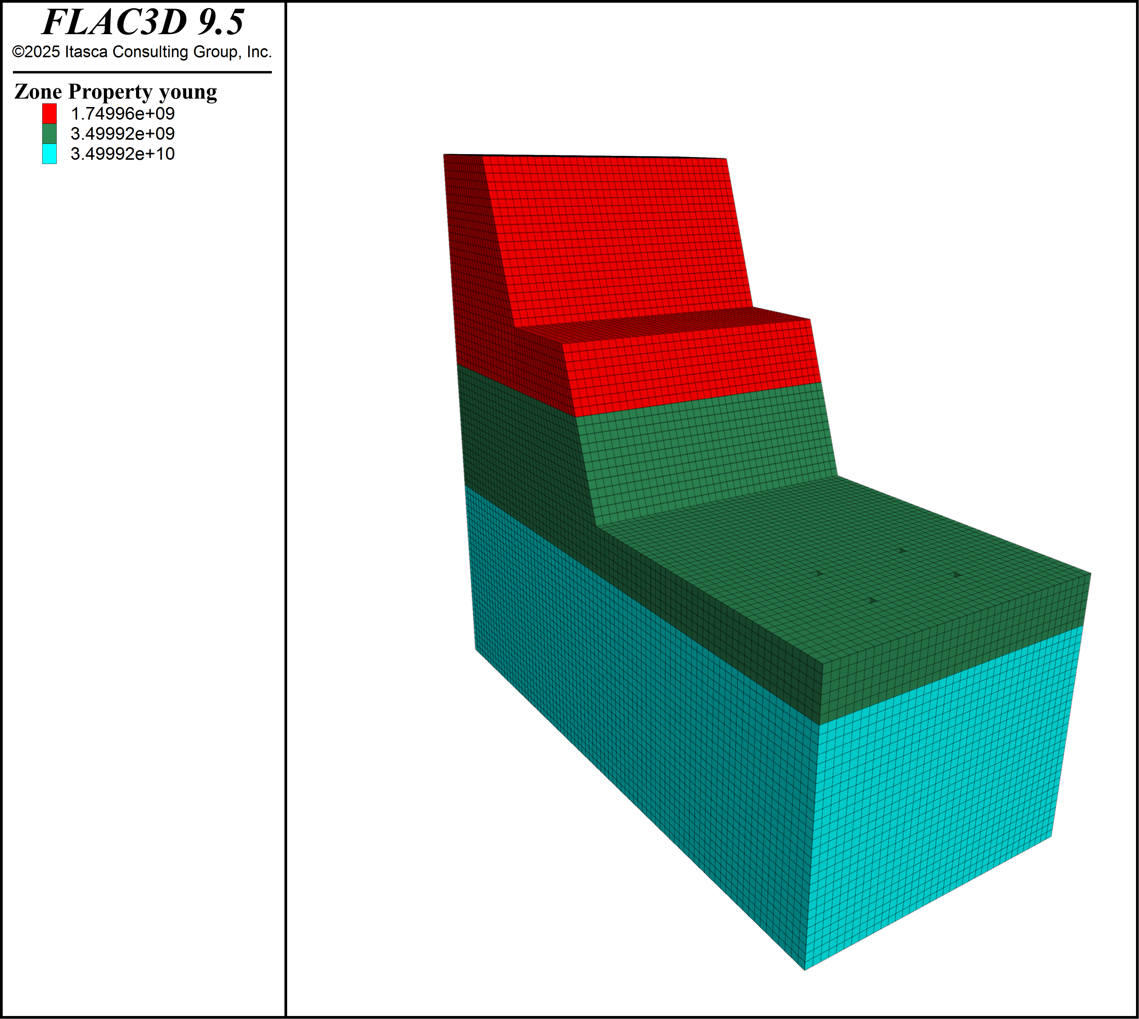
Figure 1: Model configuration.
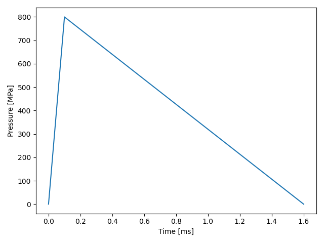
Figure 2: Simplified applied pressure wave form.
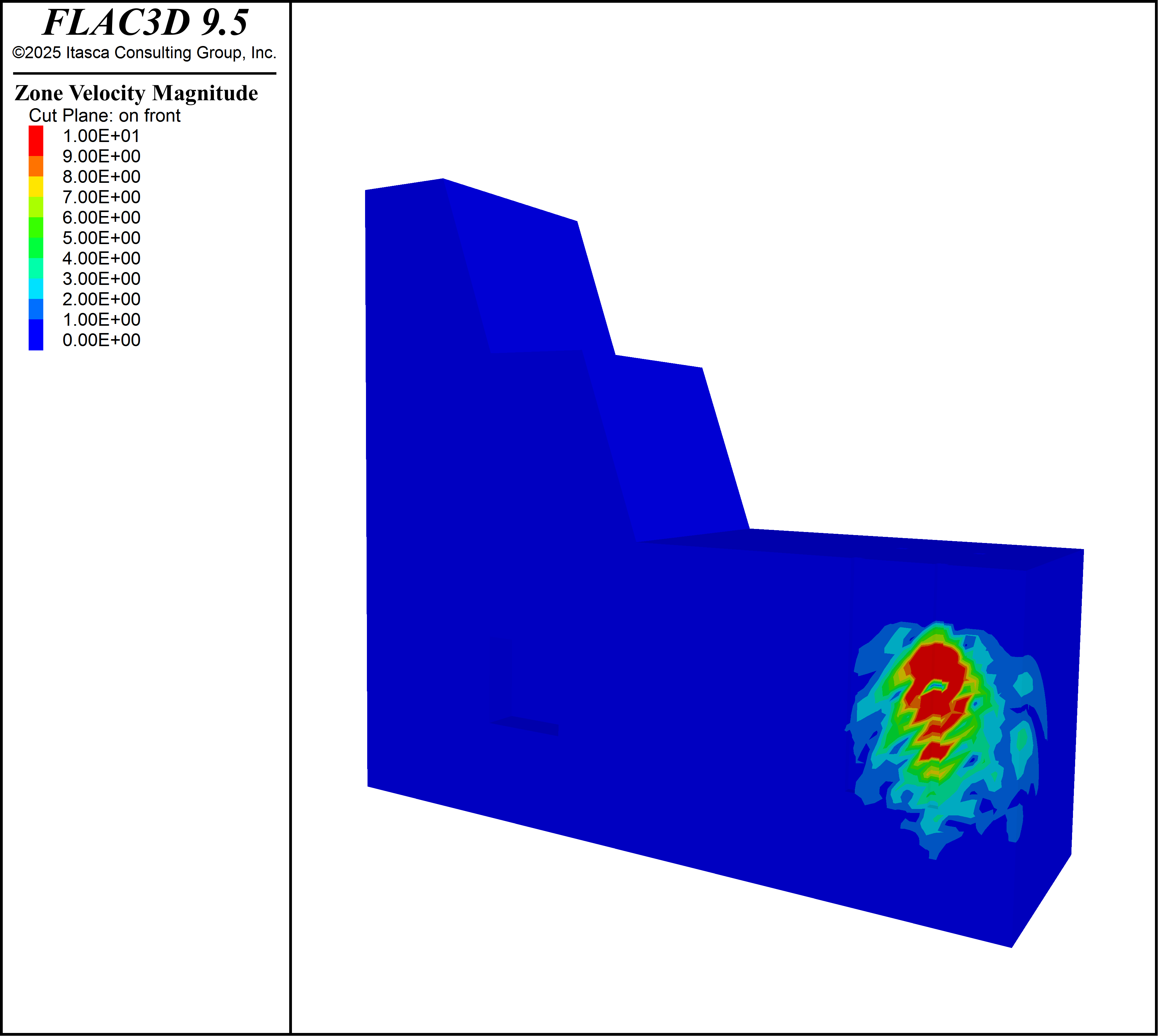
Figure 3: Gridpoint velocity magnitude on a cross-section of the model at a time near the end of detonation of the first hole.
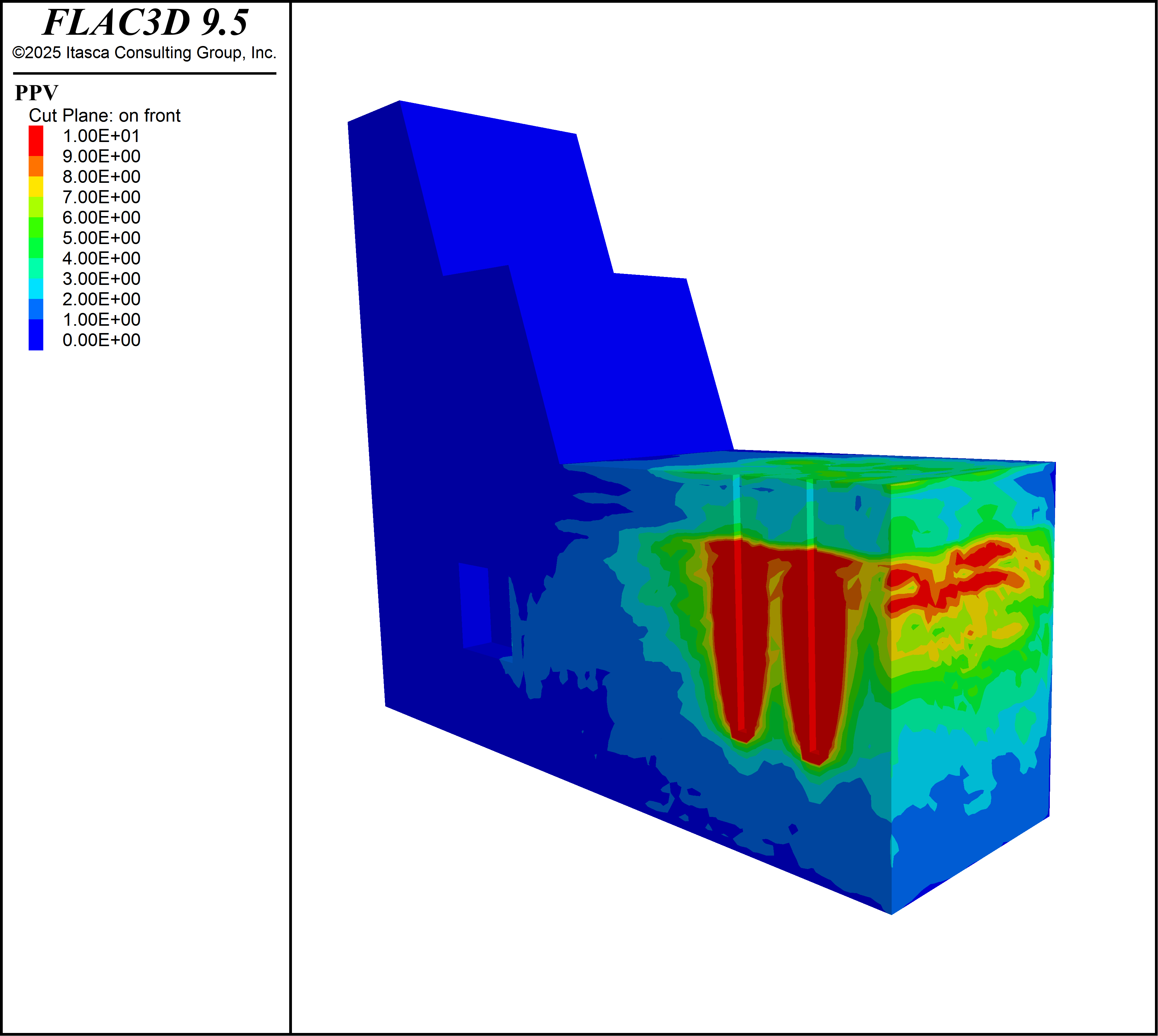
Figure 4: Gridpoint PPV at the end of the model time.
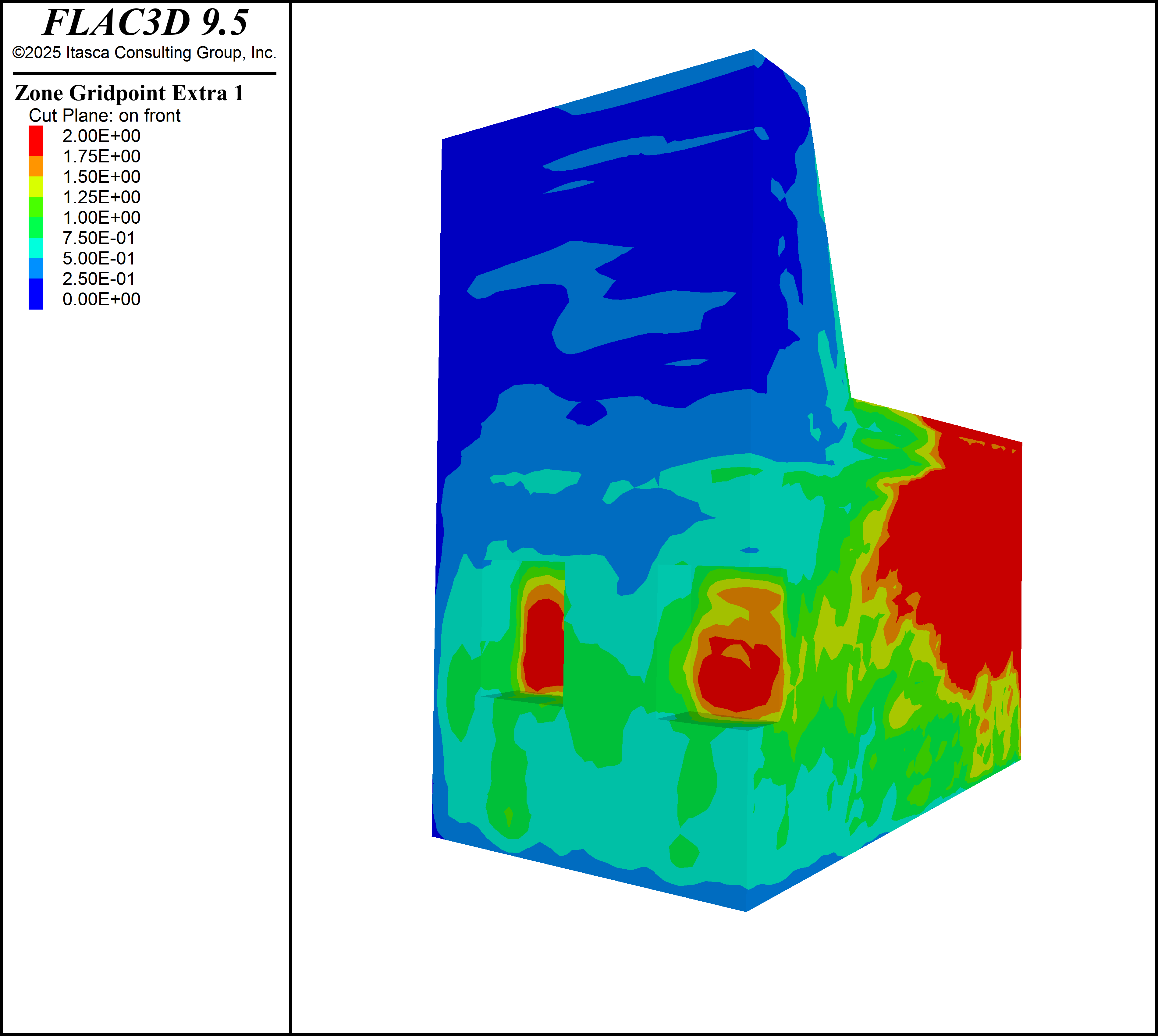
Figure 5: Gridpoint PPV on the stopes.
Data Files
geometry.py
from IPython import get_ipython; get_ipython().magic('reset -sf')
import itasca as it
from itasca import gridpointarray as gpa
from itasca import gridpoint as gp
from math import sqrt, radians, sin, cos, tan
import numpy as np
it.command("-python-reset-state false")

density = 2650
bulk = 23.33e9
shear = 14e9
E = bulk*shear*9/(3*bulk+shear)
nu = (3*bulk-2*shear)/(2*(3*bulk+shear))


hole_depth = 11.0
stemming = 4

burden = 4.0
spacing = 6.0

nhxp = 2  # number of production holes along x-direction []
nhyp = 2  # number of production holes along y-direction []

standoff =  burden *3 # standoff between production holes and toe of upper bench [m]


tzs = 0.5  # target zone size [m]
width = int((nhxp+1)*spacing)+0.5
bench_height = hole_depth -1
face_angle = 70.0
upper_length = 10
lower_length = standoff  + nhxp * burden

dx = bench_height / tan(radians(face_angle))

it.command(f"""
model new
model configure dynamic
model large-strain off
zone create brick point 0 0 0 {-hole_depth / 2.0} ...
                  point 1 {upper_length} 0 {-hole_depth / 2.0} ...
                  point 2 0 {width} {-hole_depth / 2.0} ...
                  point 3 0 0 {hole_depth} ...
                  size {int(upper_length // tzs)} {int(width // tzs)} {int((3 * hole_depth / 2.0) // tzs)}

zone create brick point 0 {upper_length} 0 {-hole_depth / 2.0} ...
                  point 1 {upper_length + lower_length} 0 {-hole_depth / 2.0} ...
                  point 2 {upper_length} {width} {-hole_depth / 2.0} ...
                  point 3 {upper_length} 0 {hole_depth} ...
                  size {int(lower_length // tzs)} {int(width // tzs)} {int((3 * hole_depth / 2.0) // tzs)}

zone create brick point 0 0 0 {hole_depth} ...
                  point 1 {upper_length} 0 {hole_depth} ...
                  point 2 0 {width} {hole_depth} ...
                  point 3 0 0 {hole_depth + bench_height} ...
                  point 4 {upper_length} {width} {hole_depth} ...
                  point 5 0 {width} {hole_depth + bench_height} ...
                  point 6 {upper_length - dx} 0 {hole_depth + bench_height} ...
                  point 7 {upper_length - dx} {width} {hole_depth + bench_height} ...
                  size {int(upper_length // tzs)} {int(width // tzs)} {int(bench_height // tzs)}

zone create brick point 0 {-upper_length} 0 {-hole_depth / 2.0} ...
                  point 1 0 0 {-hole_depth / 2.0} ...
                  point 2 {-upper_length} {width} {-hole_depth / 2.0} ...
                  point 3 {-upper_length} 0 {hole_depth + bench_height} ...
                  size {int(upper_length // tzs)} {int(width // tzs)} {int((3 * hole_depth / 2.0 + bench_height) // tzs)}

zone create brick point 0 {-upper_length} 0 {hole_depth + bench_height} ...
                  point 1 0 0 {hole_depth + bench_height} ...
                  point 2 {-upper_length} {width} {hole_depth + bench_height} ...
                  point 3 {-upper_length} 0 {hole_depth + 2.0 * bench_height} ...
                  point 4 0 {width} {hole_depth + bench_height} ...
                  point 5 {-upper_length} {width} {hole_depth + 2.0 * bench_height} ...
                  point 6 {-dx} 0 {hole_depth + 2.0 * bench_height} ...
                  point 7 {-dx} {width} {hole_depth + 2.0 * bench_height} ...
                  size {int(upper_length // tzs)} {int(width // tzs)} {int(bench_height // tzs)}
""")

hwp = (width - (nhyp - 1) * spacing) / 2.0

explosive_points = []
for i in range(nhxp):
    for j in range(nhyp):
        ex = upper_length + standoff + tzs / 2 + burden * i
        ey = width - (nhyp - 1) * spacing - hwp + spacing * j
        it.command(f"""
        zone delete range position-x {ex} position-y {ey} position-z 0 {hole_depth}
        """)
        for k in range(int((hole_depth - stemming) / tzs)): # depth index
            ez = tzs*k + 0.5*tzs
            explosive_points.append((ex,ey,ez))


# excavate stopes
it.command("""
zone delete range position-x 0 5 position-y 4 8 position-z 0 5
zone delete range position-x 0 5 position-y 12 16 position-z 0 5
""")


it.command(f"""
zone face skin
zone cmodel assign elastic
zone property density {density} young {E} poisson {nu}
zone property density {0.9*density} young {0.1*E} poisson {nu} range position-z 8 17
zone property density {0.8*density} young {0.05*E} poisson {nu} range position-z 17 100
""")

it.command(f'''
history delete
model history dynamic time-total
model save 'StaticSol.sav'
''')
blast.py
import os, shutil
zone = it.zone.find(1)

# diagonal length from bottom of holes to top of upper bench
diagonal_length = sqrt(
    (hole_depth + bench_height) ** 2
    + width ** 2
    + (lower_length + upper_length) ** 2
)

# calculate P-wave and S-wave velocities
p_wave_velocity = sqrt((zone.prop("bulk") + 4.0 / 3.0 * zone.prop("shear")) / zone.density())
s_wave_velocity = sqrt(zone.prop("shear") / zone.density())
max_p_wave_time = diagonal_length / p_wave_velocity

print("P-wave speed", p_wave_velocity)
print("S-wave speed", s_wave_velocity)
print("max P-wave time", max_p_wave_time)

ppv = None

def store_ppv():
    global ppv
    if ppv is None:
        ppv = np.zeros(gp.count())
    ppv = np.maximum(np.linalg.norm(gpa.vel(), axis=1), ppv)
    if it.cycle() % 10 == 0:
        gpa.set_extra(1, ppv)


it.set_callback("store_ppv", 0.1)


it.command(f'''
model dynamic active on
zone gridpoint free velocity-x
zone gridpoint free velocity-y
zone gridpoint free velocity-z

zone gridpoint initialize displacement-x 0.
zone gridpoint initialize displacement-y 0.
zone gridpoint initialize displacement-z 0.

zone face apply quiet range position-z {-hole_depth / 2.0}
zone face apply quiet range position-x {-upper_length}
zone face apply quiet range  position-y 0.
zone face apply quiet range  position-y {width}

zone dynamic damping rayleigh 1 1e5 stiffness
''')


nseq = nhyp // 2 + nhxp  # number of timing sequences []

# generates V chevron timing sequence in dictionary based on number of holes selected in x and y directions
timing = {}
for i in range(nseq):
    timing[i + 1] = set()

first = nhyp * nhxp - nhyp // 2
for i in range(nhxp):
    for j in range(nhxp // 2 + 1):
        timing[i + 1 + j].add(first - i * nhyp + j )
        if nhyp % 2 == 0 and j == nhyp // 2:
            break
        timing[i + 1 + j].add(first - i * nhyp - j )


delay = 5e-3 # 5 ms inter hole delay (fast relative to common field practice)
VoD = 4600  # velocity of detonation of production hole [m/s]
total_delay = nseq * delay

# approximate waveform 25cm away from blasthole centerline
rise_time = 0.1e-3
decay_time = 1.5e-3
peak_pressure = 800e6

for time_seq, holes in timing.items():
    t0 = (time_seq-1)*delay
    for hole_id in holes:
        for k in range(int((hole_depth - stemming) / tzs)): # depth index
            start_time = t0 + k*tzs/VoD
            table_file = f"table_tmp_{hole_id}_{k}.txt"
            table_name = table_file[:-4]
            with open(table_file, "w") as f:
                print("time pressure", file=f)
                print("5 0", file=f)
                print("0 0", file=f)
                print(f"{start_time} 0", file=f)
                print(f"{start_time+rise_time} {peak_pressure}", file=f)
                print(f"{start_time+rise_time+decay_time} 0", file=f)
                print(f"100 0", file=f)

            it.command(f'table "{table_name}" import "{table_file}"')
            os.remove(table_file)
            if k == 0:
                it.command(f'''
                zone face apply stress-normal -1 table "{table_name}" time dynamic range group "Top{hole_id}"
                ''') # pressure to hole bottom


            it.command(f'''
            zone face apply stress-normal -1 table "{table_name}" time dynamic range group "North{hole_id}" position-z {tzs*k} {tzs*k+tzs}
            zone face apply stress-normal -1 table "{table_name}" time dynamic range group "South{hole_id}" position-z {tzs*k} {tzs*k+tzs}
            zone face apply stress-normal -1 table "{table_name}" time dynamic range group "East{hole_id}" position-z {tzs*k} {tzs*k+tzs}
            zone face apply stress-normal -1 table "{table_name}" time dynamic range group "West{hole_id}" position-z {tzs*k} {tzs*k+tzs}
            ''')


# create/clear movie frames directory
if os.path.exists('movie_frames'):
    shutil.rmtree('movie_frames')
os.makedirs('movie_frames')

# run dynamic solve and save movie frames
it.command(f'''
model save 'PreDynSol.sav'
plot 'Zones' export bitmap filename "BlastVibrations_zones.png" size 3800 3400

;plot 'Velocity_cut' movie active on interval 3 prefix 'movie_frames/'
;plot 'PPV_cut' movie active on interval 3 prefix 'movie_frames/'
;plot 'Stopes' movie active on interval 3 prefix 'movie_frames/'
;plot 'Velocity_Stopes' movie active on interval 3 prefix 'movie_frames/'


model mechanical timestep maximum 2e-5

model solve time-total {0.8*(hole_depth/VoD)}
plot 'Velocity_cut' export bitmap filename "BlastVibrations_velocity_cut.png" size 3800 3400
plot 'Velocity_Stopes' export bitmap filename "BlastVibrations_velocity_stopes.png" size 3800 3400


model solve time-total {total_delay + max_p_wave_time }

plot 'PPV_cut' export bitmap filename "BlastVibrations_ppv_cut.png" size 3800 3400
plot 'PPV_Stopes' export bitmap filename "BlastVibrations_ppv_stopes.png" size 3800 3400


model save 'DynSol.sav'
''')

# store final PPV data
vibration_plot.py
import itasca as it
from collections import defaultdict
from scipy.spatial import KDTree
from math import pi, sqrt, log10
import pylab as plt


plt.ioff()
fig = plt.figure()
plt.plot([0,rise_time*1e3, (rise_time+decay_time)*1e3], [0, peak_pressure/1e6,0])
plt.xlabel("Time [ms]")
plt.ylabel("Pressure [MPa]")
plt.tight_layout()
plt.savefig("time_pressure_loading.png")
plt.close(fig)

gp_skin = dict()

for z in it.zone.list():
    for i in range(6):
        skin_group = z.face_group(i, "Skin")
        if skin_group:
            for gp in z.faces()[i]:
                gp_skin[gp.id()] = skin_group


face_names = {"East9": (0,"Lower bench face"),
              "Top9": (1,"Lower bench top"),
              "East8": (2,"Middle bench face"),
              "Top8": (3,"Middle bench top"),
              "East7": (4,"Top bench face"),
              "Top7": (5,"Top bench top"),
              "West5": (6,"Stope front"),
              "West6": (6,"Stope front"),
              "East5": (7,"Stope rear"),
              "East6": (7,"Stope rear"),
              "South5": (8,"Stope side"),
              "South6": (8,"Stope side"),
              "North5": (8,"Stope side"),
              "North6": (8,"Stope side")}

gp_group_names = {9: "Body lower", 10: "Body middle",
                  11: "Body top", 12:"skip"}
for n, name in face_names.values():
    gp_group_names[n]=name


gp_group = []
for gp in it.gridpoint.list():
    # skip boundary points
    if gp.pos().y() == 0:
        gp_group.append(12)
        continue
    if gp.pos().y() == width:
        gp_group.append(12)
        continue
    if gp.pos().x() == -hole_depth/2:
        gp_group.append(12)
        continue
    if gp.id() in gp_skin and gp_skin[gp.id()] in face_names:
        gp_group.append(face_names[gp_skin[gp.id()]][0])
    else:
        if gp.pos().z() > 17:
            gp_group.append(11)
        elif gp.pos().z() > 8:
            gp_group.append(10)
        else:
            gp_group.append(9)
gp_group = np.array(gp_group)

explosive_density = 776
sqrt_explosive_mass = sqrt(pi*0.1**2*(hole_depth-stemming)*explosive_density)

tree = KDTree(explosive_points)
# for each gridpoint, fund the distance ot the nearest explosive
distance, _ = res = tree.query(gpa.pos())
gpa.set_extra(2, distance/sqrt_explosive_mass)

xlim = (0.02, 4)
ylim = (14, 12_000)

# PPV scaled distance model for comparison
A = 209
ppv_c = 250
b = -1.6
sd0, sd1 = xlim
sdPPV_0 = A*(sd0)**b
sdPPV_1 = A*(sd1)**b


plt.ioff()
fig = plt.figure()
ax = plt.gca()
ax.set_xlim(xlim)
ax.set_ylim(ylim)
ax.set_xscale('log')
ax.set_yscale('log')
plt.xlabel("Scaled distance [m/$\sqrt{kg}$]")
plt.ylabel("PPV [mm/s]")

for i in [11,10,9,8,7,6,5,4,3,2,1,0]:
    mask = gp_group==i
    plt.plot(gpa.extra(2)[mask], ppv[mask]*1e3, '.', label=gp_group_names[i])
plt.legend()
plt.plot([sd0, sd1],[sdPPV_0, sdPPV_1], color="black")
plt.axhline(ppv_c, linestyle="--", color="black")
plt.tight_layout()
plt.savefig("PPV_all.png")
plt.close(fig)

fig = plt.figure()
ax = plt.gca()
ax.set_xlim(xlim)
ax.set_ylim(ylim)
ax.set_xscale('log')
ax.set_yscale('log')
plt.xlabel("Scaled distance [m/$\sqrt{kg}$]")
plt.ylabel("PPV [mm/s]")
for i in [9,10,11]:
    mask = gp_group==i
    plt.plot(gpa.extra(2)[mask], ppv[mask]*1e3, '.', label=gp_group_names[i])
plt.legend()
plt.plot([sd0, sd1],[sdPPV_0, sdPPV_1], color="black")
plt.axhline(ppv_c, linestyle="--", color="black")
plt.tight_layout()
plt.savefig("PPV_interior.png")
plt.close(fig)

fig = plt.figure()
ax = plt.gca()
ax.set_xlim(xlim)
ax.set_ylim(ylim)
ax.set_xscale('log')
ax.set_yscale('log')
plt.xlabel("Scaled distance [m/$\sqrt{kg}$]")
plt.ylabel("PPV [mm/s]")
for i in range(6):
    mask = gp_group==i
    plt.plot(gpa.extra(2)[mask], ppv[mask]*1e3, '.', label=gp_group_names[i])
plt.legend()
plt.plot([sd0, sd1],[sdPPV_0, sdPPV_1], color="black")
plt.axhline(ppv_c, linestyle="--", color="black")
plt.tight_layout()
plt.savefig("PPV_surfaces.png")
plt.close(fig)

fig = plt.figure()
ax = plt.gca()
ax.set_xlim(xlim)
ax.set_ylim(ylim)
ax.set_xscale('log')
ax.set_yscale('log')
plt.xlabel("Scaled distance [m/$\sqrt{kg}$]")
plt.ylabel("PPV [mm/s]")
for i in [6,7,8]:
    mask = gp_group==i
    plt.plot(gpa.extra(2)[mask], ppv[mask]*1e3, '.', label=gp_group_names[i])
plt.legend()
plt.plot([sd0, sd1],[sdPPV_0, sdPPV_1], color="black")
plt.axhline(ppv_c, linestyle="--", color="black")
plt.tight_layout()
plt.savefig("PPV_stopes.png")
plt.close(fig)
Endnote
| Was this helpful? ... | Itasca Software © 2024, Itasca | Updated: Nov 23, 2025 |
