Programmed Burn Method

The project file for this example may be viewed/run in FLAC2D.[1] The main data file used is shown at the end of this example.

How To Read and Use Examples

Problem Statement

The programmed burn algorithm is a numerical technique commonly used in modeling of rock blasting to simulate the detonation behavior of explosives. Unlike reactive flow models that solve complex equations governing detonation front propagation, the programmed burn method adopts a simplified approach to initiate and propagate the explosive reaction. In this method, the arrival time of the detonation front is not calculated dynamically but is instead “programmed” into the model by specifying the velocity of detonation (\(VoD\)) and the detonation point. This approach allows for efficient simulation of large-scale blasting operations without the overhead of reactive flow models. The key features are as follows.

The initial detonation point is known and specified in the model.
The velocity of detonation (\(VoD\)) is known and constant.
Upon arrival of the detonation front, the explosive is instantaneously converted to reaction product gases and exerts pressure on the surrounding rock.

This method is particularly useful in large-scale models where the primary goal is to evaluate the effects of blasting on rock masses (e.g., crushing, fracturing, vibration, stemming interaction, etc.) rather than capturing the small-scale details of the detonation shock front.

This example builds upon the One-Dimensional Explosive-Rock Interaction example by extending the model to two dimensions and capturing detonation front propagation up the borehole. This example also incorporates stemming to confine the explosive energy within the borehole.

Model Geometry

This example demonstrates the programmed burn algorithm in a 2D axisymmetric model, capturing a slice of the cylindrical geometry (Figure 1). The model extends vertically from below the bottom of the borehole to the ground surface. The borehole is explicitly modeled with a radius of 7.5 cm and represented by several zones in the vertical direction (single zone in radial direction). The borehole consists of explosive and stemming. The surrounding rock is modeled out to a radius of 8 m to capture the explosive-rock interaction. Between the borehole and the surrounding rock, an interface is used with zero shear stiffness and zero strength to allow for vertical expansion of the explosive zones, i.e., the upward flow of detonation reaction product gases. Stemming zones that are ejected upward past the top of the model are nulled with the FLAC2D command zone null.

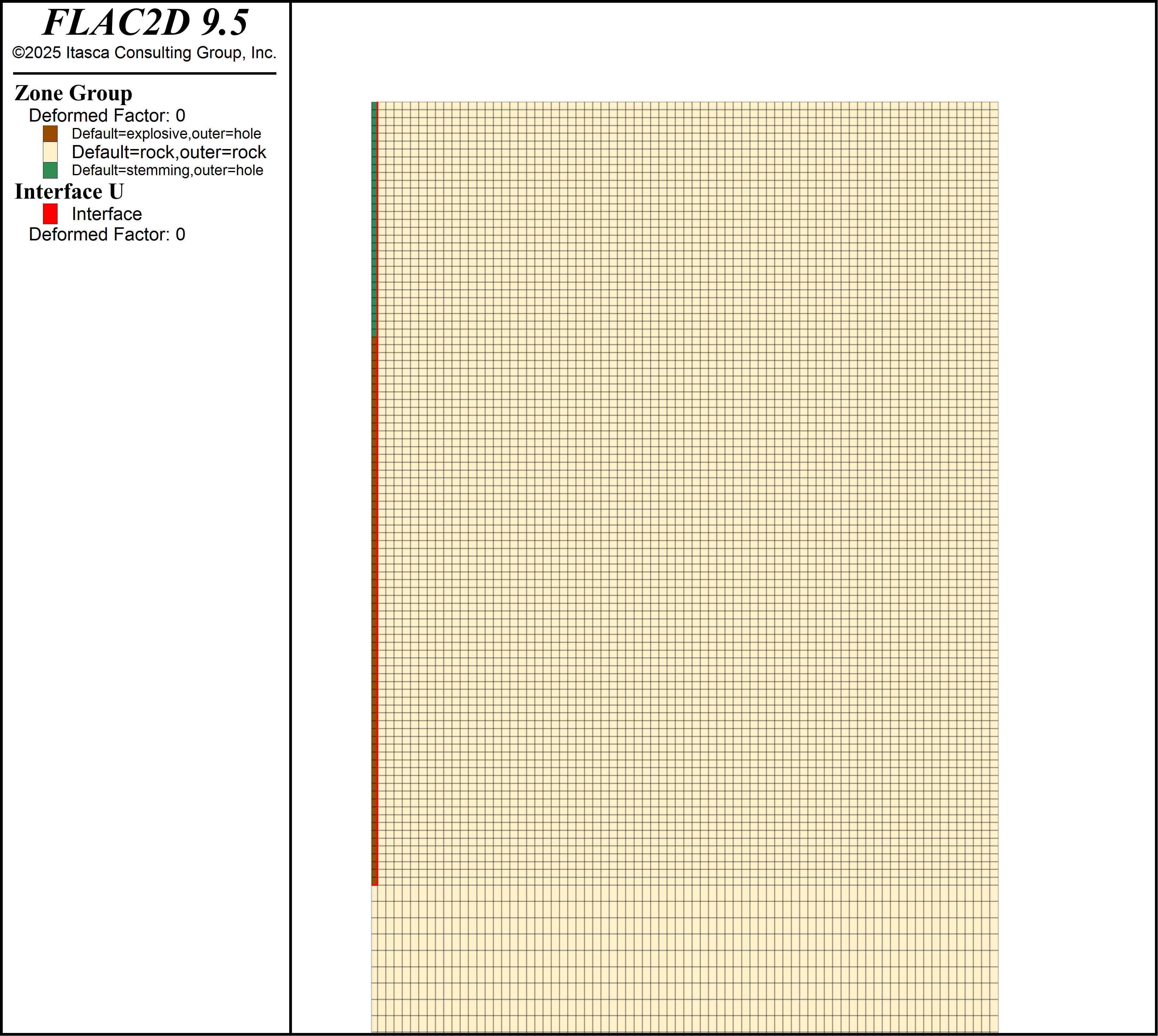
../../../../../_images/programburn_groups.png — Figure 1: Axisymmetric model geometry.

Material Properties

The explosive (ANFO) is modeled with the Jones-Wilkins-Lee (JWL) equation of state while the stemming and rock are modeled with the Mohr-Coulomb constitutive model. The stemming stiffness and strength are taken as a fraction of the surrounding rock stiffness and strength. The stemming Poisson’s ratio is, however, increased to provide resistance to upward movement. The material properties are:

Table 1: Explosive Properties (JWL model)
Property	Value	Unit
constant \(A\)	203.582	GPa
constant \(B\)	2.973	GPa
constant \(C\)	0.389	GPa
constant \(R_1\)	6.651
constant \(R_2\)	1.127
constant \(\omega\)	0.390
initial density \(\rho_0\)	776	kg/m³
detontation velocity \(VoD\)	4048	m/s

Table 2: Rock and Stemming Properties (Mohr-Coulomb model)
Property	Rock	Stemming	Unit
density \(\rho\)	3000	1500	kg/m³
Young’s modulus \(E\)	35	3.5	GPa
Poisson’s ratio \(\nu\)	0.25	0.35
friction angle \(\phi\)	55	55	\(^\circ\)
cohesive strength \(c\)	23.5	2.35	MPa

A Note on Hourglass Resistance

As discussed in the Jones-Wilkins-Lee (JWL) constitutive model, the Lagrangian frame of reference combined with zero shear resistance and gigapascal pressures has the potential to create non-physical hourglass deformation mode in JWL zones. In this example, a viscous damping force is applied to all nodes within the explosive zones to suppress the hourglass deformation mode. A simple method involves penalizing the nodes with velocity opposite in direction to the average zone velocity:

(1)\[F_{hg}^{node} = \sum_{zone=1}^{n} - K_{hg} \left(v^{node} - v^{zone}\right) L_{r}^{zone}\]

where \(F_{hg}^{node}\) is the nodal force added to global equilibrium, \(K_{hg}\) is the viscous damping coefficient (on the order of \(10^6\)), \(v^{node}\) is the nodal velocity, \(v^{zone}\) is the average velocity of the zone, and \(L_{r}^{zone}\) is an aspect ratio coefficient between opposite sides of the quadrilateral zones. The aspect ratio coefficient is defined such that the nodal damping force is zero when the aspect ratio is unity and increases linearly as the zone geometry deforms in an hourglass shape:

(2)\[L_{r}^{zone} = |1 - \frac{\Delta x_1}{\Delta x_2}|\]

where \(\Delta x_1\) and \(\Delta x_2\) are the lengths of opposite sides of quadrilateral zones and \(\Delta x_1 < \Delta x_2\). For example, \(\Delta x_1\) corresponds to the facet length of the top, bottom, left, or right facet. The nodal force vector is assembled following standard Finite Element procedure, i.e., outer loop over elements and inner loop over nodes. These equations are implemented in Python and set as a callback during cycling. The Python function is shown at the end of this example. Other methods including selective hourglass velocity filtering and stiffness proportional damping are available in the literature.

Results

The time history of borehole radial displacement and plastic deformation are discussed in One-Dimensional Explosive-Rock Interaction example. The present results discussion focuses on two dimensional effects not seen in that one-dimensional model.

The results are shown at two times, first the model state when the detonation wave is halfway through the explosive and second after detonation has completed and the strong dynamic effects have ended. Figure 2 shows the contours of gridpoint velocity in the model at the halfway time. Note the Mach cone observed at an angle of 33 degrees from the vertical, this angle is equal to 0.5 asin(Vp/VoD). Figure 3 shows a closeup of the vertical component of velocity around the detonation front, note the upward vertical velocity of around 600 m/s. The sliding interface allows the reaction product gas to move upward in the borehole.

Peak particle velocity (PPV) is the maximum velocity vector magnitude seen at a given location during a blast. This is often used as a metric for damage and fragmentation. A Python function tracks the PPV at each gridpoint and there is a function to interpolate these values onto the zone centroids. Figure 4 shows the PPV at the end of the model run. There is a region of high PPV around the explosive which decreases with radial distance away, there is an amplification effect due to reflection at the free surface. PPV can be a proxy for local fragmentation size and rock damage.

Radial displacement at the borehole wall for two locations is shown in Figure 5. The borehole radius is initially 7.5 cm and expands to 15 cm after crushing and fracturing of the adjacent rock. Location of the displacement histories are given in the data files at the end of this example.

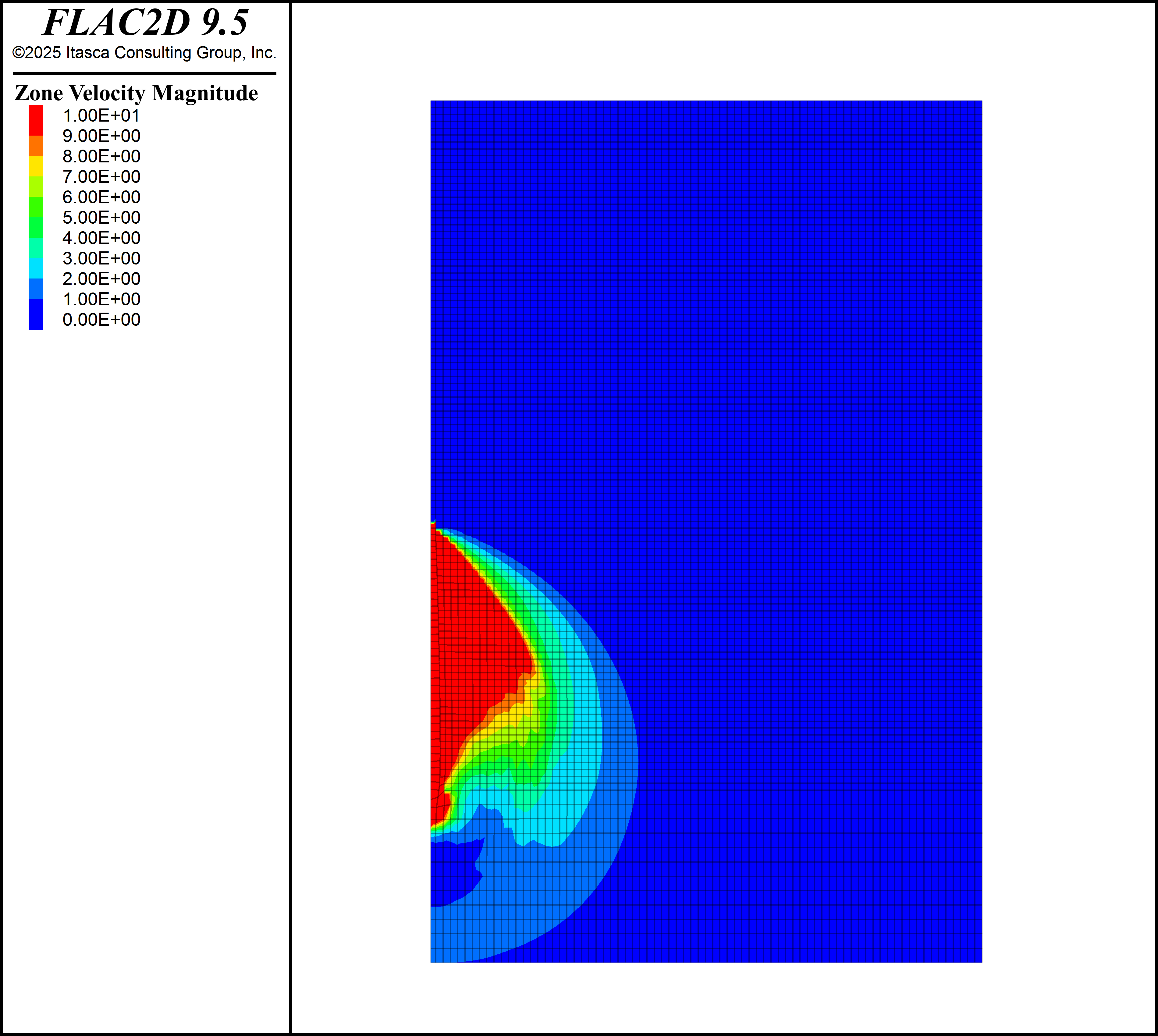
../../../../../_images/programburn_velocity_mid.png — Figure 2: Velocity at the halfway time.

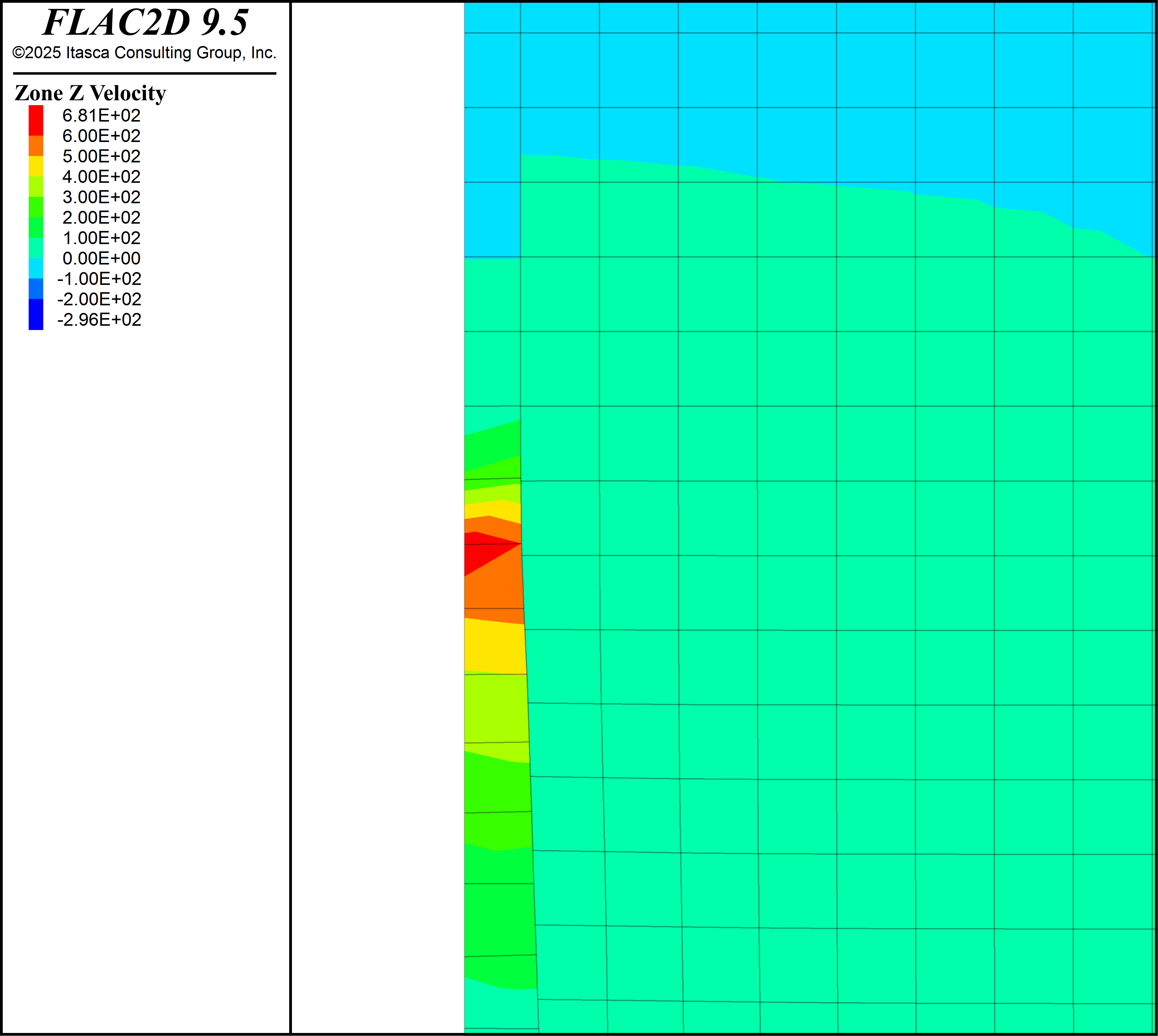
../../../../../_images/programburn_velocity_mid_close.png — Figure 3: Close-up of the detonation front velocity at the halfway time.

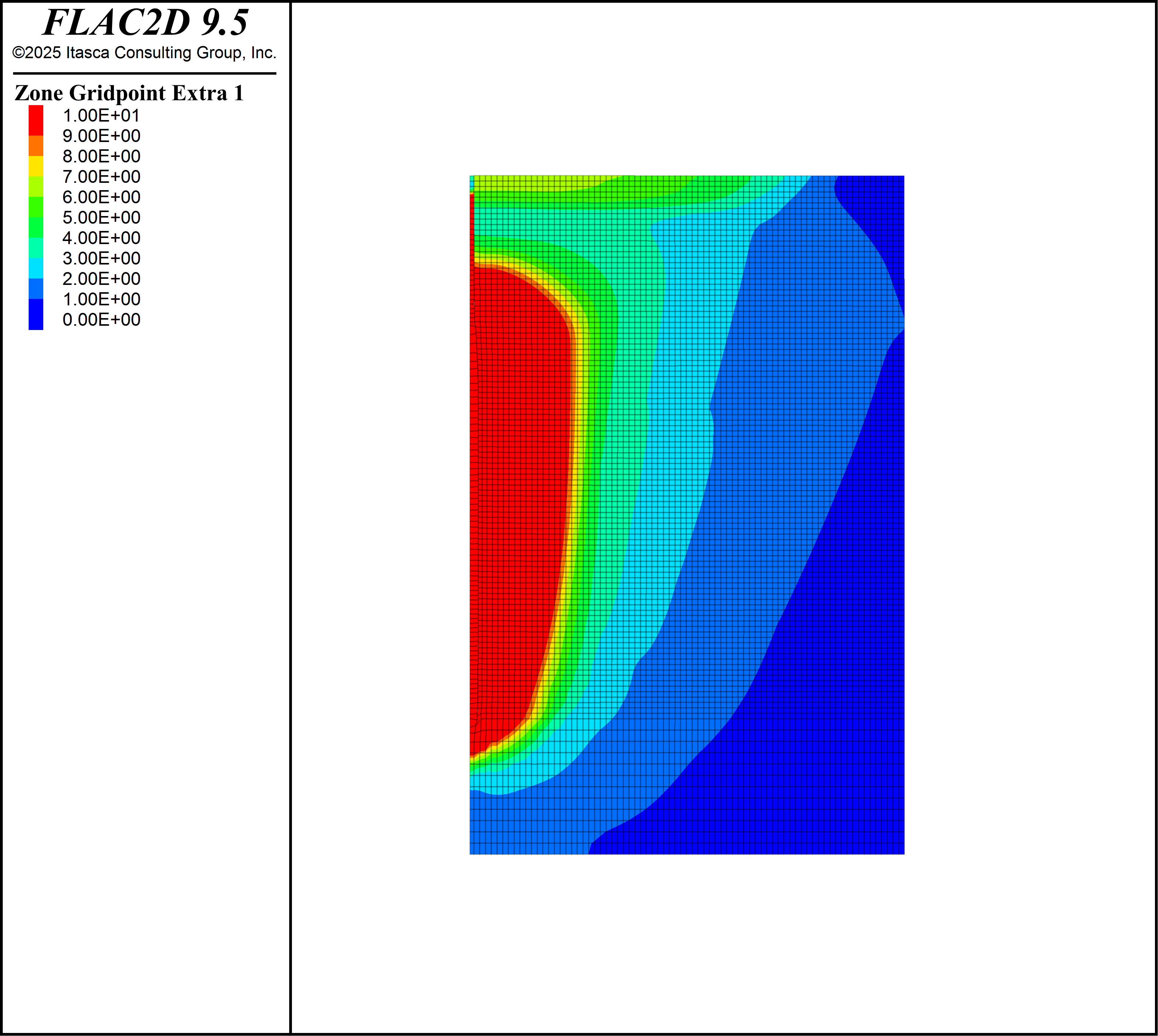
../../../../../_images/programburn_ppv.png — Figure 4: Peak particle velocity (PPV) at the model end time.

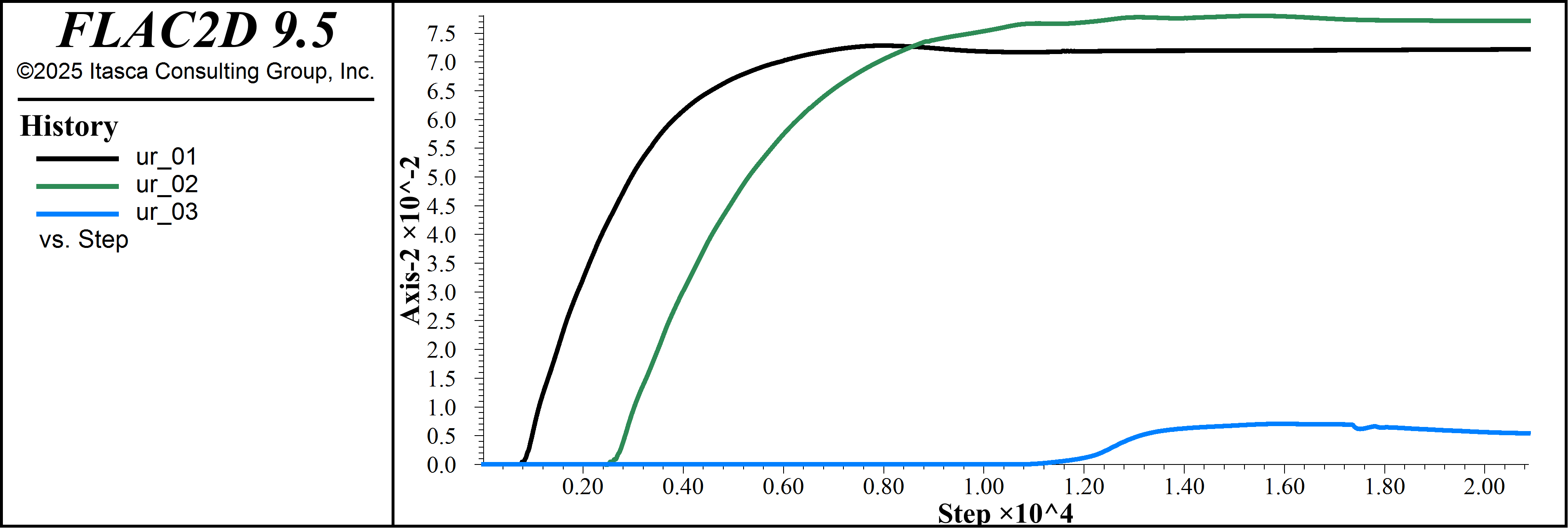
../../../../../_images/programburn_disp.png — Figure 5: Radial displacement.

Data Files

blast.dat

;------------------------------------------------;
; Physical constants
;------------------------------------------------;
[hole_radius = 0.075]
[out_radius = 8.0]

[charge_height = 7]
[stemm_height = 3]

[ny = 100]
[nx = 75]

[total_height = charge_height+stemm_height]
[charge_ny = int(ny*charge_height/total_height)]
[stemm_ny = int(ny*stemm_height/total_height)]
[dx = out_radius/nx]

fish define explosive_params
    global a, b, c, r1, r2, omega, edens
    a = 203.582e9
    b = 2.973e9
    c = 0.389e9
    r1 = 6.651
    r2 = 1.127
    omega = 0.39
    edens = 776
    
    global VOD = 4048
end

fish define rock_params
    global rdens,young,poisson,friction,ucs
    rdens = 3000
    young = 35e9
    poisson = 0.25
    friction = 55
    ucs = 150e6
    
    global q,cohesion,tension
    local fric_rad = friction*math.pi/180.0
    q = (1.0+math.sin(fric_rad)) / (1.0-math.sin(fric_rad))
    cohesion = ucs/(2.0*math.sqrt(q))
    tension = 0.1*cohesion
    
    global bulk,shear,Vp,tmax
    bulk = young/(3*(1-2*poisson))
    shear = young/(2*(1+poisson))
    Vp = math.sqrt((bulk+4/3*shear)/rdens)
    Vs = math.sqrt(shear/rdens)
    tmax = 1.5*out_radius/Vp
    tmid = charge_height/2/VOD
end

fish define stemm_params
    global sdens,syoung,spoisson
    sdens = 0.5*rdens
    syoung = 0.1*young
    spoisson = 0.35
    
    global sucs,sq,scohesion,sfriction,stension
    sfriction = 55
    sucs = 0.1*ucs
    local fric_rad = sfriction*math.pi/180.0
    sq = (1.0+math.sin(fric_rad)) / (1.0-math.sin(fric_rad))
    scohesion = sucs/(2.0*math.sqrt(sq))
    stension = 0.1*scohesion
end

[explosive_params]
[rock_params]
[stemm_params]

;------------------------------------------------;
; Model geometry
;------------------------------------------------;
zone create quadrilateral size 1 [charge_ny] ...
    point 0 (0, 0) point 1 ([hole_radius], 0) ...
    point 2 (0, [charge_height]) point 3 ([hole_radius],[charge_height]) ...
    group "hole" slot "outer"
    
zone create quadrilateral size [nx] [charge_ny] ...
    point 0 ([hole_radius], 0) point 1 ([out_radius], 0) ...
    point 2 ([hole_radius], [charge_height]) point 3 ([out_radius],[charge_height]) ...
    group "rock"
    
zone create quadrilateral size 1 [stemm_ny] ...
    point 0 (0, [charge_height]) point 1 ([hole_radius], [charge_height]) ...
    point 2 (0, [total_height]) point 3 ([hole_radius],[total_height]) ...
    group "hole" slot "outer"
    
zone create quadrilateral size [nx] [stemm_ny] ...
    point 0 ([hole_radius], [charge_height]) point 1 ([out_radius], [charge_height]) ...
    point 2 ([hole_radius], [total_height]) point 3 ([out_radius],[total_height]) ...
    group "rock"
    
zone create quadrilateral size [nx] [int(ny/4/2)] ...
    point 0 ([hole_radius] [-total_height/4]) point 1 ([out_radius], [-total_height/4]) ...
    point 2 ([hole_radius], 0) point 3 ([out_radius], 0) ...
    group "rock"

zone create quadrilateral size 1 [int(ny/4/2)] ...
    point 0 (0, [-total_height/4]) point 1 ([hole_radius], [-total_height/4]) ...
    point 2 (0, 0) point 3 ([hole_radius], 0) ...
    group "rock"


zone group "explosive" range position-x 0 [hole_radius] position-y 0 [charge_height]
zone group "stemming" range position-x 0 [hole_radius] position-y [charge_height] 1e12
zone group "rock" slot 'outer' range group "rock"

[xmin = list.min(zone.pos(::zone.list)->x)]
[ymin = list.min(zone.pos(::zone.list)->y)]
[det_pos = vector(xmin,hole_radius/2)]
[Zp_det = zone.near((xmin,hole_radius/2))]

;------------------------------------------------;
; Constitutive models
;------------------------------------------------;
zone cmodel assign mohr-coulomb range group "rock"
zone property density [rdens] young [young] poisson [poisson] ...
    cohesion [cohesion] tension [tension] range group "rock"
    
zone cmodel assign mohr-coulomb range group "stemming"
zone property density [sdens] young [syoung] poisson [spoisson] ...
    cohesion [scohesion] tension [stension] range group "stemming"
    
zone cmodel assign jones-wilkins-lee range group "explosive"
zone property density [edens] initial-density [edens] a [a] ...
    b [b] c [c] r-1 [r1] r-2 [r2] omega [omega] range group "explosive"

zone mechanical energy active true
program floating-point-check false


;------------------------------------------------;
; Sliding interface (borehole wall)
;------------------------------------------------;
zone interface name "sliding" create by-face separate range ...
    group "hole" group "rock" slot "outer"
zone interface name "sliding" node property stiffness-normal [10*young/dx] ...
    stiffness-shear 0 friction 33.0 tension 0



;------------------------------------------------;
; Boundary conditions
;------------------------------------------------;
zone gridpoint fix velocity-x range position-x 0
zone face apply quiet range position-x [out_radius]
zone face apply quiet range position-y [-total_height/4]

zone dynamic damping rayleigh 1 1e5 stiffness
zone dynamic safety-factor 1.3

;------------------------------------------------;
; Histories
;------------------------------------------------;
program call "functions.py" suppress

zone history name "s3_01" stress quantity maximum position ...
    ([0.10*out_radius],[0.25*total_height])
zone history name "s3_02" stress quantity maximum position ...
    ([0.50*out_radius],[0.25*total_height])
zone history name "s3_03" stress quantity maximum position ...
    ([0.75*out_radius],[0.25*total_height])
    
zone history name "s1_01" stress quantity minimum position ...
    ([0.10*out_radius],[0.25*total_height])
zone history name "s1_02" stress quantity minimum position ...
    ([0.50*out_radius],[0.25*total_height])
zone history name "s1_03" stress quantity minimum position ...
    ([0.75*out_radius],[0.25*total_height])
    
zone history name "ur_01" displacement-x position ...
    ([hole_radius], [0.1*total_height])
zone history name "ur_02" displacement-x position ...
    ([hole_radius], [0.25*total_height])
zone history name "ur_03" displacement-x position ...
    ([hole_radius], [0.75*total_height])

model save 'pre_solve.sav'

;------------------------------------------------;
; Solve
;------------------------------------------------;
fish define solve_loop
    global time = 0.0
    global dt = 5e-5
    
    loop while (time < tmid)
        time += dt
        command
            zone null range position-y [total_height] 1e12
            model solve time-total [time]
        endcommand
        
        local per_done = (time / tmax) * 1.0e2
        io.out(string.build("Model completion: %1", per_done))
    endloop
    command
      model save "mid_detonation.sav"
    endcommand
    loop while (time < tmax)
        time += dt
        command
            zone null range position-y [total_height] 1e12
            model solve time-total [time]
        endcommand
        
        per_done = (time / tmax) * 1.0e2
        io.out(string.build("Model completion: %1", per_done))
    endloop    
    
end

[solve_loop]

functions.py

Endnote

⇄

⇐ One-Dimensional Explosive-Rock Interaction | Three-Dimensional Vibrations ⇒

Was this helpful? ...

Updated: Sep 09, 2025