One-Dimensional Explosive-Rock Interaction

Example Application

The project file for this example may be viewed/run in FLAC2D.[1] The main data file used is shown at the end of this example. The model in this example was used to train the explosive rock interaction rapid tool.

How To Read and Use Examples

Problem Statement

This example illustrates the application of the Jones-Wilkins-Lee (JWL) equation of state constitutive model to analyze the explosive-rock interaction near a blasthole. It builds upon the Single-Zone JWL Pressurization example, extending the analysis to explicitly model the surrounding rock as an elastoplastic medium.

The interaction between explosives and rock is a dynamic process involving transfer of energy into the rock, leading to a sequence of mechanical responses including crushing, fracturing, fragmentation, and vibrations (Figure 1). Detonation of explosives induces stress waves that propagate radially into the surrounding rock. The stress waves quickly attenuate with distance, transitioning from a high amplitude compressive wave (crushed zone) to a lower amplitude tensile wave (fractured zone). The transition between the two zones is controlled largely by the rock’s mechanical properties and the explosive type. Beyond the initial tensile fracturing zone, the rock breaks down into discrete fragments. The size distribution of the fragments is often modeled using empirical relationships that depend on rock properties, explosive properties, and geometrical parameters, e.g., Kuz-Ram.

Figure 1: Illustration of blasting induced rock crushing and fragmentation. The symbol \(\sigma_T\) refers to tensile hoop stress induced by large compressive stresses in the crushed zone.

This example approximates a one-dimensional radial response around a blasthole as a two-dimensional axisymmetric domain that represents a slice of the full cylindrical geometry. The model geometry is shown in Figure 2. The explosive is modeled with a single quadrilateral zone (FLAC2D command zone create quadrilateral) of radius and height of 0.1 m. The surrounding rock is modeled with several zones that begin at a radius of 0.1 m and extend 200 times the initial hole radius. The explosive (ANFO) and rock properties are given in Tables 1 and 2, respectively.

Figure 2: FLAC2D axisymmetric model geometry, groups, and stress history locations. The model geometry approximates an axisymmetric response around the cylindrical explosive charge.

Energy release within the explosive is controlled by a constant burn fraction set to unity for the model duration, implying instantaneous and complete detonation at time \(t=0\) s. The total model run time is \(t_{max}=0.95 L/V_p\), where \(L\) is the the model length in the radial direction and \(V_p\) is the rock P-wave velocity. A large domain relative to the borehole size and a time factor of 0.95 ensures that the induced stress wave passes through the entire model and the model stops just before the wave reaches the outer boundary. A small quantity of broad frequency stiffness proportional Rayleigh damping is applied to all zones with center frequency of \(10^5\) Hz. Most energy reduction with distance is due to the geometric effects of cylindrical and spherical divergence, but some inelastic energy dissipation is added via damping.

Table 1: Explosive Properties (JWL model)

Property	Value	Unit
constant \(A\)	203.582	GPa
constant \(B\)	2.973	GPa
constant \(C\)	0.389	GPa
constant \(R_1\)	6.651
constant \(R_2\)	1.127
constant \(\omega\)	0.390
initial density \(\rho_0\)	800	kg/m3

These coefficients are from [Sanchidrián2015].

Table 2: Rock Properties (Mohr-Coulomb model)

Property	Value	Unit
density \(\rho\)	2650	kg/m3
bulk modulus \(K\)	23.33	GPa
shear modulus \(G\)	14	GPa
friction angle \(\phi\)	37	degrees
cohesive strength \(c\)	12.5	MPa
tensile strength \(\sigma^t\)	2.5	MPa

Results

Figures 3 and 4 show time histories of pressure and expanded hole radius within the explosive zone. Explosive pressure increases rapidly to 1.6 GPa at the onset of detonation, this is the explosion pressure state when the explosive has detonated completely and is at the original density. The pressure then decreases as radial expansion occurs. The pressure stabilizes to 170 MPa by the end of the model run time. This represents the equilibrium pressure state when the expanded reaction product gases are in equilibrium with the elastic and plastic deformation in the rock — before fractures allow for gas flow and the burden starts to move. The hole starts at 200 mm in diameter and is 350 mm in diameter at the equilibrium state. Furthermore, Figure 5 shows the time histories of maximum principal stress (elasticity sign convention, least compressive) at select locations within the rock. The stress histories show large compressive stresses nearby the explosive that attenuate quickly with distance and become tensile at later times. This is consistent with the idealized crushing and fracturing processes shown in Figure 1. Lastly, the model states at the end of the simulation are shown in Figure 6. Shear failure (crushing) occurs nearby the explosive, driven by large increase in compressive stresses. Further away, the rock is failed in tension (fracturing) due to the tensile hoop stresses reaching the tensile strength of the rock. A mixed failure mode is observed in the intermediate region, where both shear and tensile failure occur. The model results are consistent with the expected behavior of explosive-rock interaction. Finally, Figure 7 shows the pressure at 25 cm from the hole centerline, this pressure time history is used as a starting point for the Three dimensional vibrations example.

Further calculations are done in the file energy.py to show conversion of the explosive potential energy to other forms of energy. During the detonation reaction, more than half the chemical potential energy is irreversibly converted into heat energy. These blasting models are isothermal as the blasting effects occur fast relative to the timescales of heat transfer. The remaining expansion potential energy is determined by evaluating the integral p dV, where p is pressure and V is volume of the reaction product gas. The integration range is from the explosion state (original density) to an expanded volume near atmospheric pressure. The explosive in this case has 2.2 MJ/kg of expansion energy density. For this explosive, hole diameter, and rock properties: 62% of the energy is dissipated in plastic flow (crushing the rock), 6% escapes the borehole region as vibrations, 4% is converted into the kinetic energy of the moving burden, and 28% is vented to the atmosphere via gas expansion. The burden is throw at a velocity of 6 m/s. The burden throw model is described in [Furtney2012].

Figure 3: Pressure within the explosive vs. time.

Figure 4: Expanded radius of the explosive vs. time. Original hole radius is 0.1 m.

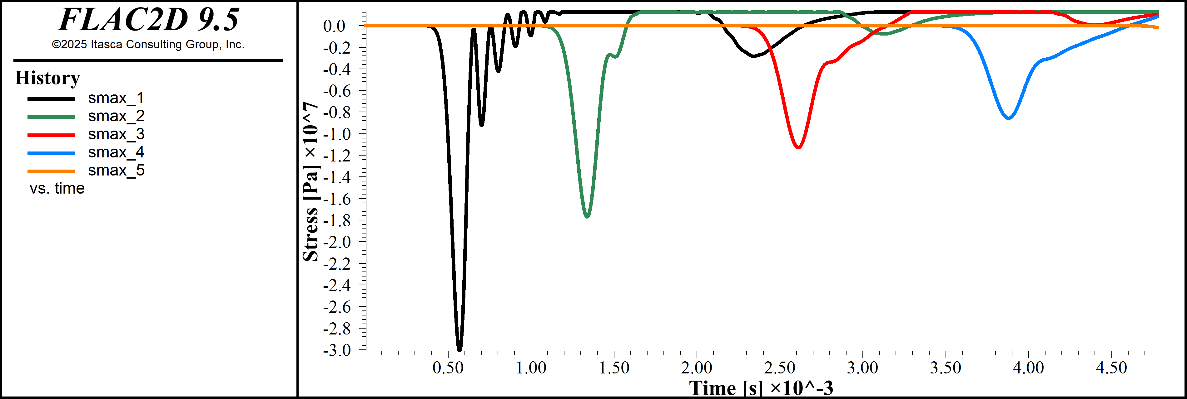
Figure 5: Maximum principal stress (least compressive) histories at select locations.

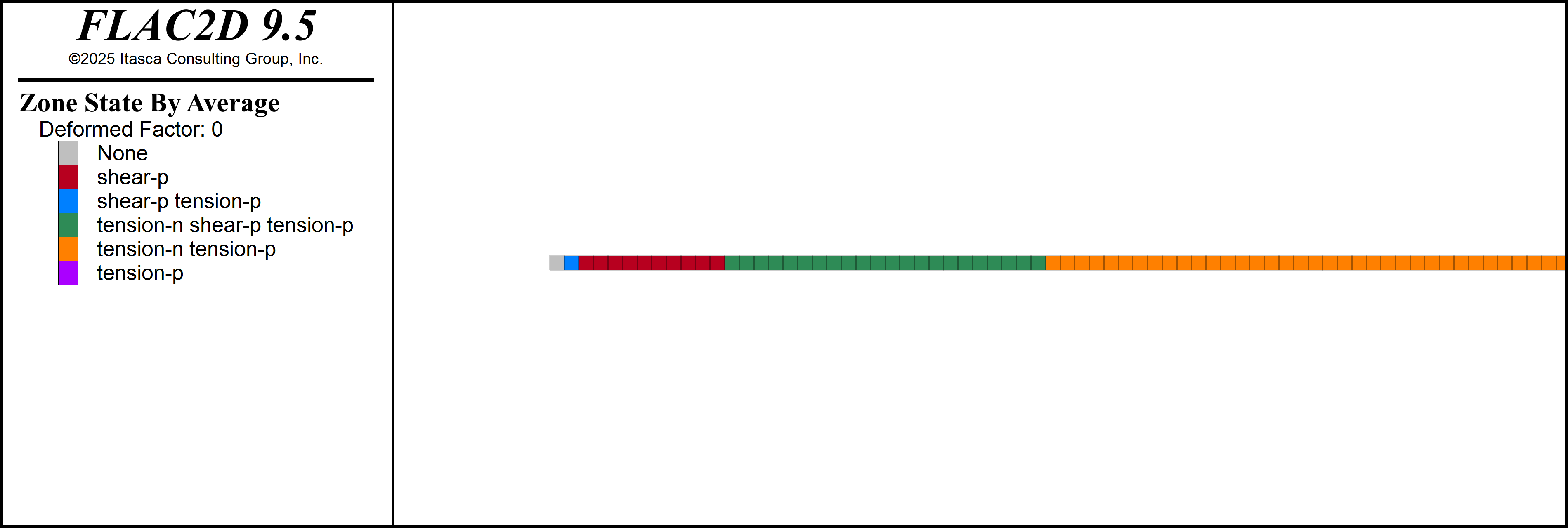
Figure 6: Model states at the end of the simulation.

Figure 7: Model states at the end of the simulation.

References

[Furtney2012]

Furtney, J. K., E. Sellers and I. Onederra. (2012) Simple Models for the Complex Process of Rock Blasting, in Rock Fragmentation by Blasting: Fragblast 10 (Proceedings, 10th International Symposium on Rock Fragmentation by Blasting, New Delhi, November 2012), pp. 275-282, P. K. Singh and A. Sinha, Eds. London, UK: CRC Press/Balkema, 2012.

[Sanchidrián2015]

Jose A. Sanchidrián, Ricardo Castedo, Lina M. López, Pablo Segarra, Anastasio P. Santos, (2015) Determination of the JWL Constants for ANFO and Emulsion Explosives from Cylinder Test Data, Central European Journal of Energetic Materials, 2015, 12(2), 177-194.

Data Files

blast.dat

[r = 0.1]
[L = 200*r]

program call "properties.dat"

zone create quadrilateral point 0 (0,0) ...
                          point 1 ([r],0) ...
                          point 2 (0,[r]) ...
                          size 1 1
                    
zone create quadrilateral point 0 ([r],0) ...
                          point 1 ([L+r],0) ...
                          point 2 ([r],[r]) ...
                          size [int(L/r)] 1

[gp0 = gp.near((r,0))]
[zp0 = zone.near((0,0))]

zone group "explosive" range position-x -1e12 [r]
zone group "rock" range position-x [r] 1e12
zone face skin

zone geometry update-interval 1
zone dynamic damping rayleigh 1 1e5 stiffness

zone cmodel assign jones-wilkins-lee range group "explosive"
zone cmodel assign mohr-coulomb range group "rock"

zone property density [dens] a [a] b [b] c [c] r-1 [r1] ...
    r-2 [r2] omega [omega] initial-density [dens] ...
    burn-fraction 1.0 range group "explosive"

zone property density [rdens] bulk [bulk] shear [shear] ...
    cohesion [cohesion] friction [friction] tension [tension] ...
    range group "rock"

zone face apply quiet-normal range group "East"
zone face apply quiet-tangential range group "East"
zone gridpoint fix velocity-y 0

history interval 1
model history name "time" dynamic time-total
fish history name "press" [-zone.stress(zp0)->xx]
fish history name "radius" [gp.disp(gp0)->x + r]
zone history name "smax_1" stress quantity maximum position ([0.10*L+r],0)
zone history name "smax_2" stress quantity maximum position ([0.25*L+r],0)
zone history name "smax_3" stress quantity maximum position ([0.50*L+r],0)
zone history name "smax_4" stress quantity maximum position ([0.75*L+r],0)
zone history name "smax_5" stress quantity maximum position ([1.00*L+r],0)
zone history name "smin_25cm" stress quantity minimum position (0.25, 0)

[global explosive_volume_0 = zone.area(zone.find(1))]
zone mechanical energy active true
model solve-dynamic [tmax]
model save "blast.sav"

properties.dat

fish define set_jwl_params
    global a, b, c, r1, r2, omega, dens
    a = 203.582e9
    b = 2.973e9
    c = 0.389e9
    r1 = 6.651
    r2 = 1.127
    omega = 0.39
    dens = 776
end

fish define set_rock_params
    global rdens, bulk, shear, Vp, tmax
    rdens = 2650
    bulk = 23.33e9
    shear = 14e9
    
    Vp = math.sqrt((bulk+4/3*shear)/rdens)
    tmax = 0.95*L/Vp
    
    global ucs, friction, q, cohesion, tension
    ucs = 50e6
    friction = 37.0
    
    local fric_rad = friction*math.pi/180.0
    q = (1.0+math.sin(fric_rad)) / (1.0-math.sin(fric_rad))
    cohesion = ucs/(2.0*math.sqrt(q))
    tension = 0.1*cohesion
end

[set_jwl_params]
[set_rock_params]

energy.py

import itasca as it
import numpy as np
import matplotlib; matplotlib.rcParams["savefig.directory"] = "."
from matplotlib import pyplot as plt
plt.rcParams.update({'font.size': 18})
from math import exp, pi
from scipy.interpolate import interp1d
from scipy.integrate import quad
from itasca import zonearray as za
from itasca import gridpointarray as gpa
from scipy.integrate import odeint


class JWL:
    def __init__(self, A, B, C, R1, R2, omega):
        self.A = A
        self.B = B
        self.C = C
        self.R1 = R1
        self.R2 = R2
        self.omega = omega

    def __call__(self, reducedVolume):
        V = reducedVolume
        A = self.A
        B = self.B
        C = self.C
        R1 = self.R1
        R2 = self.R2
        omega = self.omega
        P = A * exp(-R1 * V) + B * exp(-R2 * V) + C * V ** (-omega - 1)
        return P

initial_hole_radius = it.fish.get("r")
z_plastic = np.array([z.work_plastic_total() for z in it.zone.list() if not z.model()=="jones-wilkins-lee"])
zx, _ = za.pos().T
plastic_radius = float(interp1d(np.cumsum(z_plastic) / sum(z_plastic), zx[1:])(0.90))
print(f"Hole initial radius: {100*initial_hole_radius:.1f} cm" )
print(f"Expanded hole radius: {100*it.fish.get('radius'):.1f} cm" )
print(f"Crushed zone radius: {plastic_radius*100:.1f} cm" )

A,B,C,R1,R2,omega = it.fish.get("a"), it.fish.get("b"), it.fish.get("c"), it.fish.get("r1"), it.fish.get("r2"), it.fish.get("omega")

EoS = JWL(A, B, C, R1, R2, omega)
exp_density = it.fish.get("dens")
v0 = 1/exp_density
v1 = 100*v0
print(f"Explosion pressure: {EoS(1.0)/1e6:.1f} MPa")
equilibrium_pressure = -it.zone.find(1).stress().xx()/1e6
print(f"Equilibrium Pressure: {equilibrium_pressure:.1f} MPa")
exp_per_kg = quad(lambda v: EoS(v/v0), v0,v1)[0]
print(f"Explosive specific energy (for expansion work) {exp_per_kg/1e6:.1f} MJ/kg")
explosive_initial_volume = it.fish.get("explosive_volume_0")
exp_total_energy = exp_per_kg*(explosive_initial_volume*exp_density)

x, _ = gpa.pos().T
ke =  np.array([0.5 * gp.mass_gravity() * gp.vel().mag() ** 2 * gp.pos().x() for gp in it.gridpoint.list()])
ke_total = np.sum(ke)
z_elastic = np.array([z.work_elastic_total() for z in it.zone.list() if not z.model()=="jwl"])

plastic_total = np.sum(z_plastic)
elastic_total = np.sum(z_elastic)
explosive_current_volume = it.zone.find(1).vol()

E_gas = quad(lambda v: EoS(v/explosive_initial_volume), explosive_initial_volume, explosive_current_volume)[0]
explosive_gas_energy = exp_total_energy-E_gas

class simple_throw_model():
    "This is a simple model that predicts burden velocity"
    def __init__(self, EoS, rv_eq, burden, spacing, height, face_angle, stemming_length,
                 hole_radius, rock_density):
        assert stemming_length < 0.75*height
        self.stemming_length = stemming_length
        self.EoS = EoS
        self.rv_eq = rv_eq
        self.rad_0 = hole_radius
        self.hole_length = height
        self.rock_density = rock_density
        self.rad_eq = np.sqrt(self.rv_eq * self.rad_0 * self.rad_0)
        self.volume_eq = (self.hole_length - self.stemming_length) * np.pi * self.rad_eq**2
        self.burden_volume = height * burden * spacing + 0.5*spacing*height/np.tan(np.radians(face_angle))
        self.burden_mass = self.rock_density * self.burden_volume

    def solve(self, end_time=1.0):
        vf_c  = 342.0 # constants describing gas velocity as a function of burden displacement
        vf_Q  = 0.1244
        vf_B  = 3.681
        vf_M  = -0.850
        vf_nu = 2.91
        sina = np.sin(np.deg2rad(90 / 2.0))
        phi0 = 0.15
        d0   = 2 * self.rad_eq

        area = lambda x: (2 * self.rad_eq) * (self.hole_length-self.stemming_length)
        phi = lambda x: 1 - (1 - phi0) * (d0 / (x + d0))
        pressure = lambda vol: max(1e-6, self.EoS(vol / self.volume_eq * self.rv_eq) - 1e5)
        acceleration = lambda vol, x: pressure(vol) * area(x) / self.burden_mass
        vf = lambda x: 0 if x==0 else vf_c/(1+vf_Q*np.exp(-vf_B*(np.log10(sina*x)-vf_M)))**(1/vf_nu)
        dvfdt = lambda x:  self.hole_length * x * sina * vf(x)
        dvdt = lambda u: 2 * self.rad_eq * u * (self.hole_length - self.stemming_length)
        dvsdt = lambda x: vf_c * (np.pi * self.rad_eq ** 2 + 2 * self.rad_eq * x)*phi(x)
        x0 = [0.0, 0.0, self.volume_eq, 0, 0]  # initial conditions
        def deriv(x, t):
            # x is position, velocity, and cavity, fracture and stemming gas volumes
            position = x[0]
            velocity = x[1]
            v_c = x[2]
            v_f = x[3]
            v_s = x[4]
            volume = v_c + v_f + v_s
            return [velocity,
                    acceleration(volume, position),
                    dvdt(velocity),
                    dvfdt(position),
                    dvsdt(position)]

        time = [0.0] + np.logspace(-4, np.log10(end_time), 1000).tolist()

        res = odeint(deriv, x0, time)
        self.disp, self.vel = res[:, 0], res[:, 1]
        self.v_c, self.v_f, self.v_s = res[:, 2], res[:, 3], res[:, 4]
        self.vol_total = res[:, 2] + res[:, 3] + res[:, 4]
        self.pressure = [pressure(_) + 1.01e5 for _ in self.vol_total]
        self.time = np.array(time)

burden = 5
spacing = 5
height = 10
stemming_length = 4
face_angle = 90.0
throw_model = simple_throw_model(EoS,
                                 explosive_current_volume/explosive_initial_volume,
                                 burden, spacing, height, face_angle, stemming_length,
                                 initial_hole_radius, it.fish.get("rdens"))

throw_model.solve()

def get_eqtime(t, p):
    pmax = p.max()
    pend = p[-1]
    p05 = (pmax-pend)*0.025 + pend
    t05 = None
    for i in range(len(p)-1,0,-1):
        if p[i] >= p05:
            t05 = t[i]
            break
    assert t05
    return t05

flac_time = it.history.get("time")[:,1]
flac_pressure = it.history.get("press")[:,1]

eq_time = get_eqtime(flac_time, flac_pressure)*2
eq_time_index = np.argmin(np.abs(flac_time-eq_time))
flac_time = flac_time[:eq_time_index]
flac_pressure = flac_pressure[:eq_time_index]

throw_time = throw_model.time + flac_time[-1]
throw_pressure = throw_model.pressure
throw_velocity = throw_model.vel[-1]
burden_ke = 0.5*throw_velocity**2*throw_model.burden_mass
explosive_mass = initial_hole_radius **2 * pi * (height-stemming_length)
frac_burden_ke = burden_ke/exp_per_kg/explosive_mass/exp_density

print()
print(f"throw_velocity {throw_velocity:.1f} m/s")
print()
print("Explosive expansion energy distribution:")
print(f"Crushing: {100*plastic_total/exp_total_energy:.1f}%")
print(f"Vibrations: {100*(elastic_total+ke_total)/exp_total_energy:.1f}%")
print(f"Burden kinetic energy: {frac_burden_ke*100:.1f} %")
print(f"Energy lost to gas venting: {100*(explosive_gas_energy-frac_burden_ke*exp_total_energy)/exp_total_energy:.1f}%" )
print()


it.fish.set("throw_velocity", throw_velocity)
it.fish.set("plastic_energy_fraction", 100*plastic_total/exp_total_energy)


plt.ioff()
fig = plt.figure()
plt.semilogx(flac_time.tolist()+throw_time.tolist(), np.array(flac_pressure.tolist()+throw_pressure)/1e6)
plt.ylabel("Pressure [MPa]")
plt.xlabel("Time [s]")
plt.tight_layout()
plt.savefig("pressure_time25.png")
plt.close(fig)

flac_time = it.history.get("time")[:,1]
flac_pressure_25cm = it.history.get("smin_25cm")[:,1]
fig = plt.figure()
plt.plot(flac_time*1e3, -flac_pressure_25cm/1e6)
plt.ylabel("Pressure at 25 cm [MPa]")
plt.xlabel("Time [ms]")
plt.tight_layout()
plt.savefig("pressure_time25.png")
plt.close(fig)

Endnote

[1]

This example is listed under the present document title in the i Examples dialog (use the menu command Help -> Examples… to access).