Rock Blasting Throw
The project file for this example may be viewed/run in PFC3D.[1] The main data file used is shown at the end of this example.
Problem Statement
Predicting and optimizing rock movement during blasting is important to prevent unnecessary material handling, reduce ore loss and dilution, to improve safety, and to the minimize environmental footprint. This example demonstrates the use of PFC3D to model the rock blasting throw and the muckpile formation. In this model, the horizontal velocity imparted on the burden by the blast is prescribed as 4 m/s. The model begins after the rock has been fragmented and the vector direction of rock movement is set according to the inter-hole and inter-row timing pattern. Particles are fixed in place with zero velocity until the blasthole near a particle goes off and movement begins. Particles are freed and given an initial horizontal and small positive vertical component. The horizontal velocity components are determined by the local angle of the hole timing contours, in this case after the first hole all subsequent holes are initiated to move at a 45 degree angle in the +ve X +ve Y direction (North-east).
Note
In this example the horizontal velocity is prescribed as 4 m/s, the example One-Dimensional Explosive-Rock Interaction calculates a throw velocity from a blast design and rock properties. This calculation can also be done with the Explosive-Rock interaction rapid tool.
In the context of rock blasting, the angular shape of fragmented rock prevents the fragments from rotating easily, leading to interlocking behavior within the rock mass. However, this PFC3D model uses spherical particles that rotate readily. To represent rock movement during blasting, the rolling resistance linear model is used to account for the energy dissipation that occurs due to rolling resistance at the contacts between particles representing the fragments. The rolling resistance contact model incorporates a torque acting on the contacting pieces to counteract the rolling motion. The behavior of the rolling resistance linear contact model is similar to the linear model, except that the internal moment is incremented linearly with the accumulated relative rotation of the contacting pieces at the contact point. The contact model was implemented at both ball-ball contacts and ball-wall contacts.
A bench 6 m tall, 6 m deep, and 40 m wide is created. To speed up model creation, a small model is created first in periodic space with a small isotropic stress and allowed to reach equilibrium. To create the bench, this brick is duplicated in the \(x\)-, \(y\)-, and \(z\)-directions to create the desired model size. Some balls are deleted to reach the desired final shape. A box wall encloses the bench, and the newly assembled model is run to equilibrium with a small confining stress in order to break some of the periodicity induced by the brick duplication. The box wall is deleted and the contact forces are zeroed.
Table 1 shows a few key parameters that define the contact model. A comprehensive description of all parameters of the rolling resistance linear contact model is available. Note that the Young’s modulus is set to a value that is smaller than normal to optimize the simulation timestep. This value is sufficient to ensure that the system remains within the rigid grain limit (i.e., further increasing the modulus/contact stiffness would not significantly affect the results). The relatively high friction coefficient and rolling friction coefficient were used to enhance particle friction and interlocking, which can be verified by comparing with field measurements and laboratory experiments.
Parameter |
Value |
Unit |
|---|---|---|
Nominal Young’s modulus |
1e7 |
Pa |
Normal-to-shear stiffness ratio |
2 |
|
Friction coefficient |
0.5 |
|
Rolling friction coefficient |
0.5 |
A wall inclined at a 30 degree angle is created 3.5 meters away from the bench toe to represent muck from a previous blast.
Results
Starting configuration shows the initial configuration of the walls and particles before movement starts, timing shows the particles colored by the time movement begins for each particle, and start position. The model is run for 300 ms and a save state is created. Early velocity shows the particle velocity magnitude as a color contour after the first 6 sets of holes have started moving. The model is run on until all the rock has moved and a solve commands is given to let the particles come to a rest on the muck pile. Distance traveled shows a cross section of the muck with the particles colored by distance traveled. Final configuration shows the particles making up the muckpile after 4.5 seconds have elapsed.
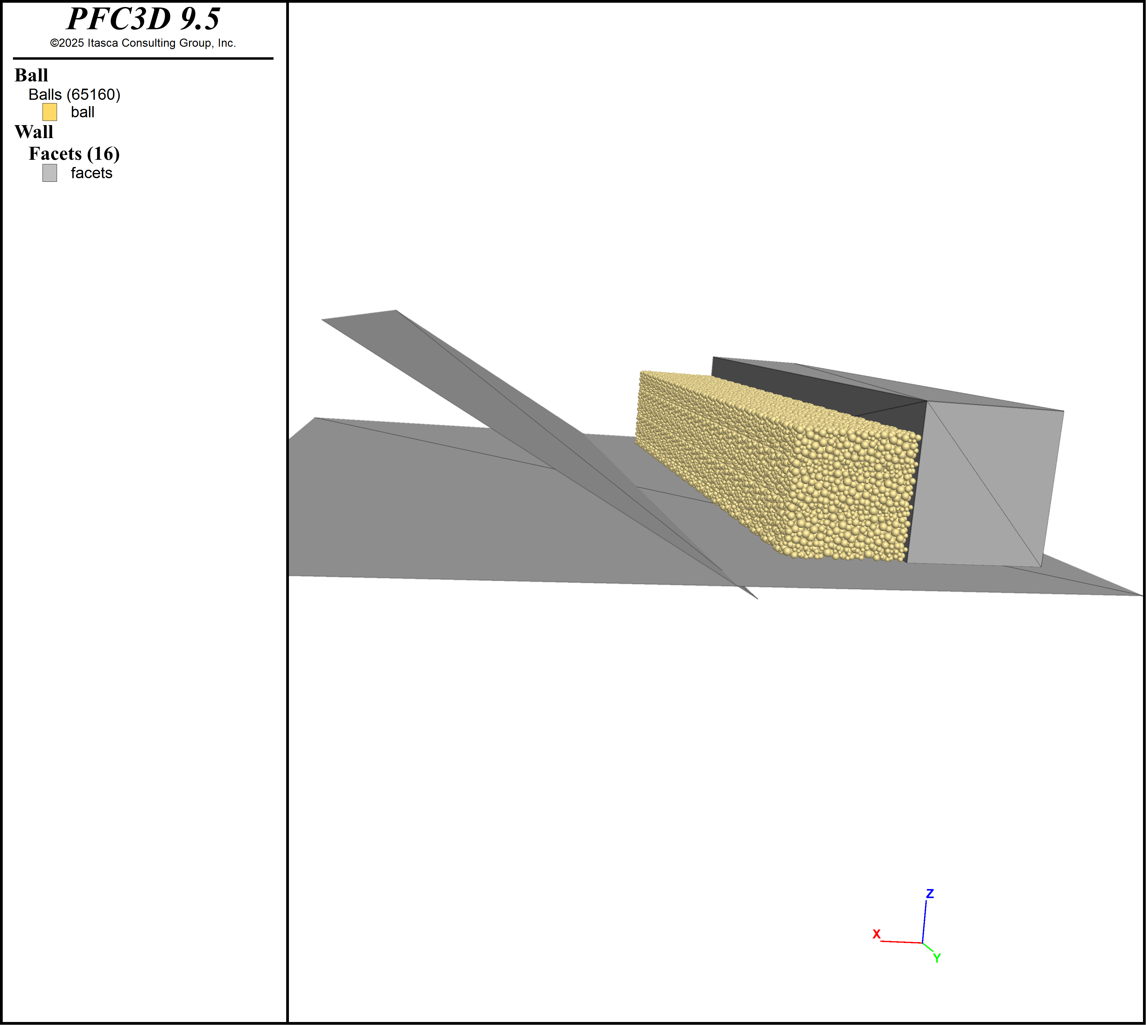
Figure 1: Starting configuration of particles and walls representing benches and previously blasted materials.
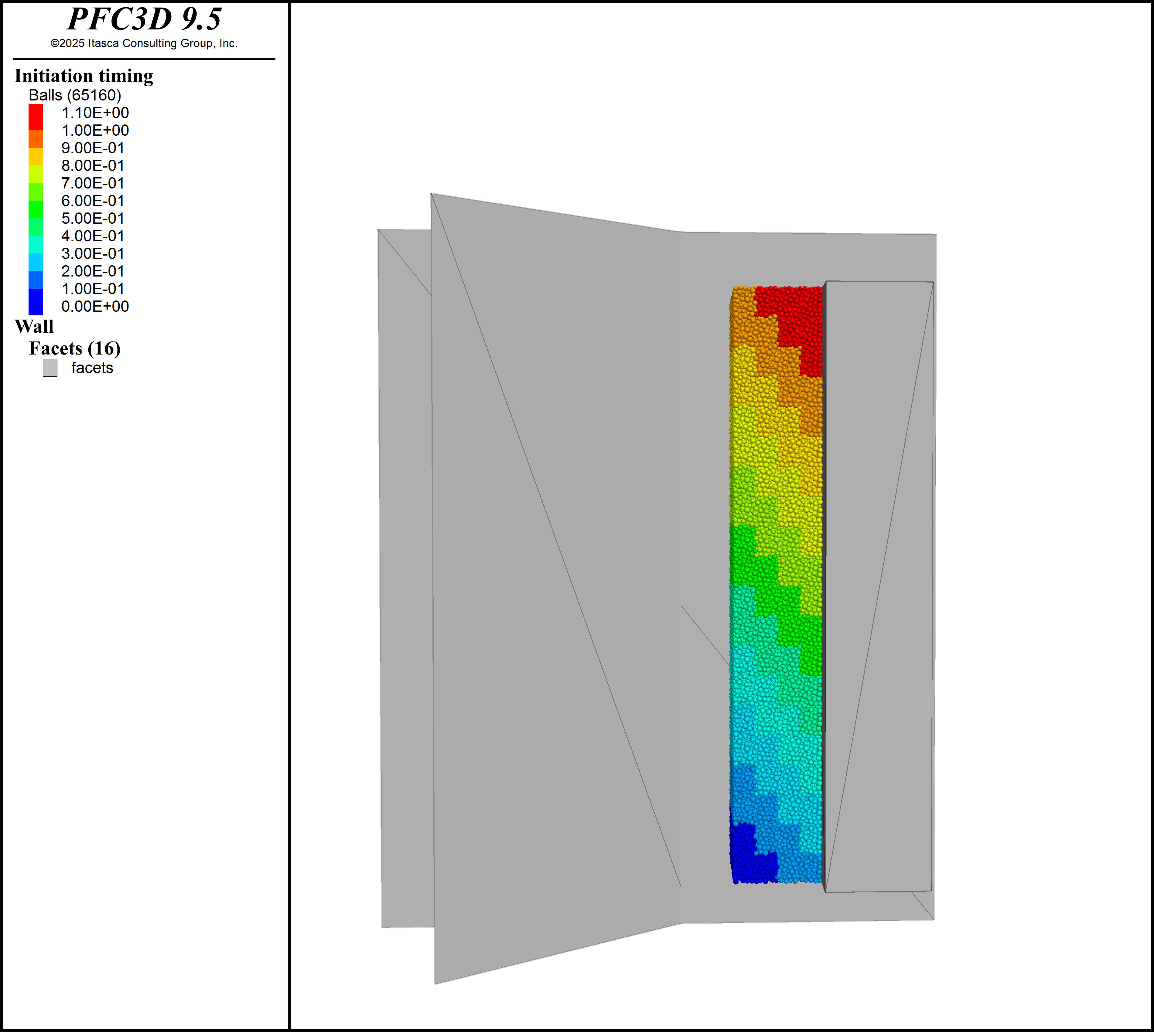
Figure 2: Particles colored by the assigned time that movement starts.
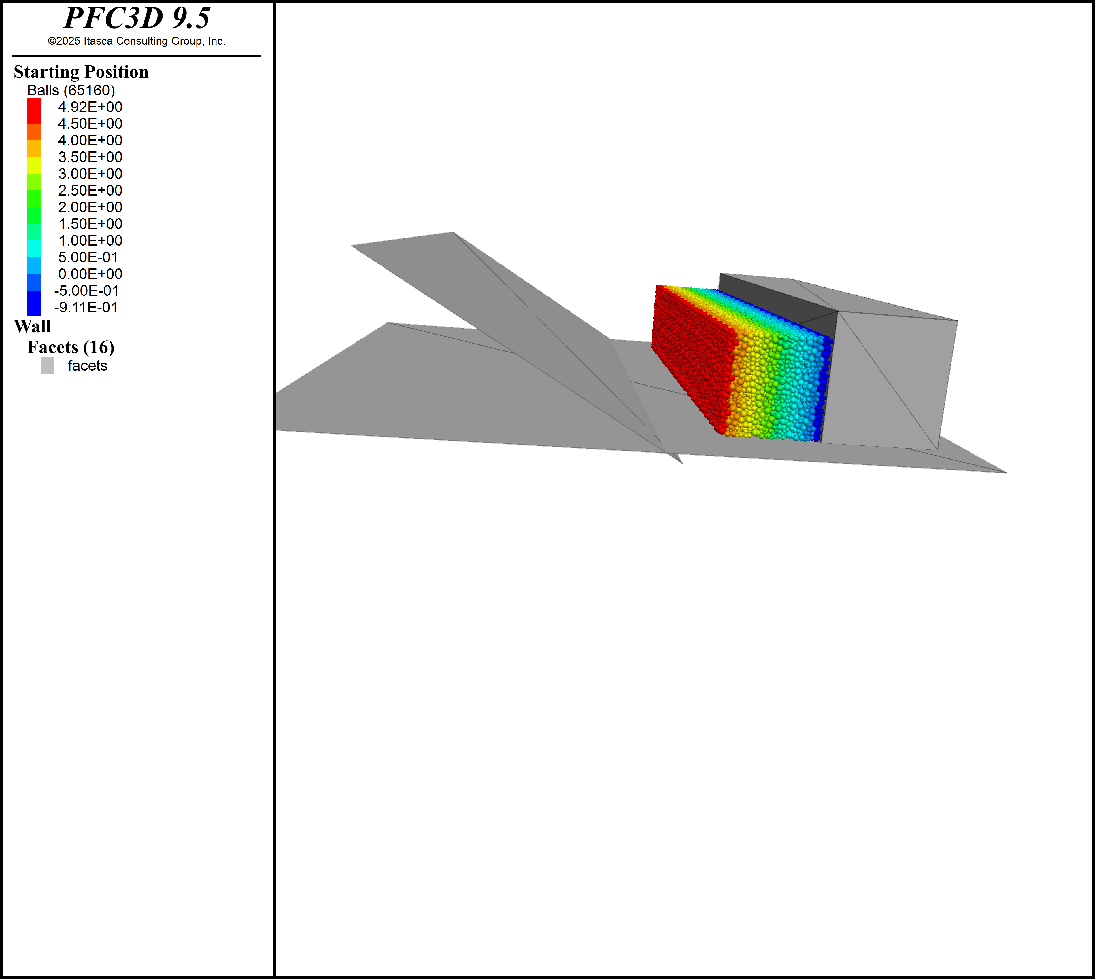
Figure 3: Particles colored by initial vertical position.
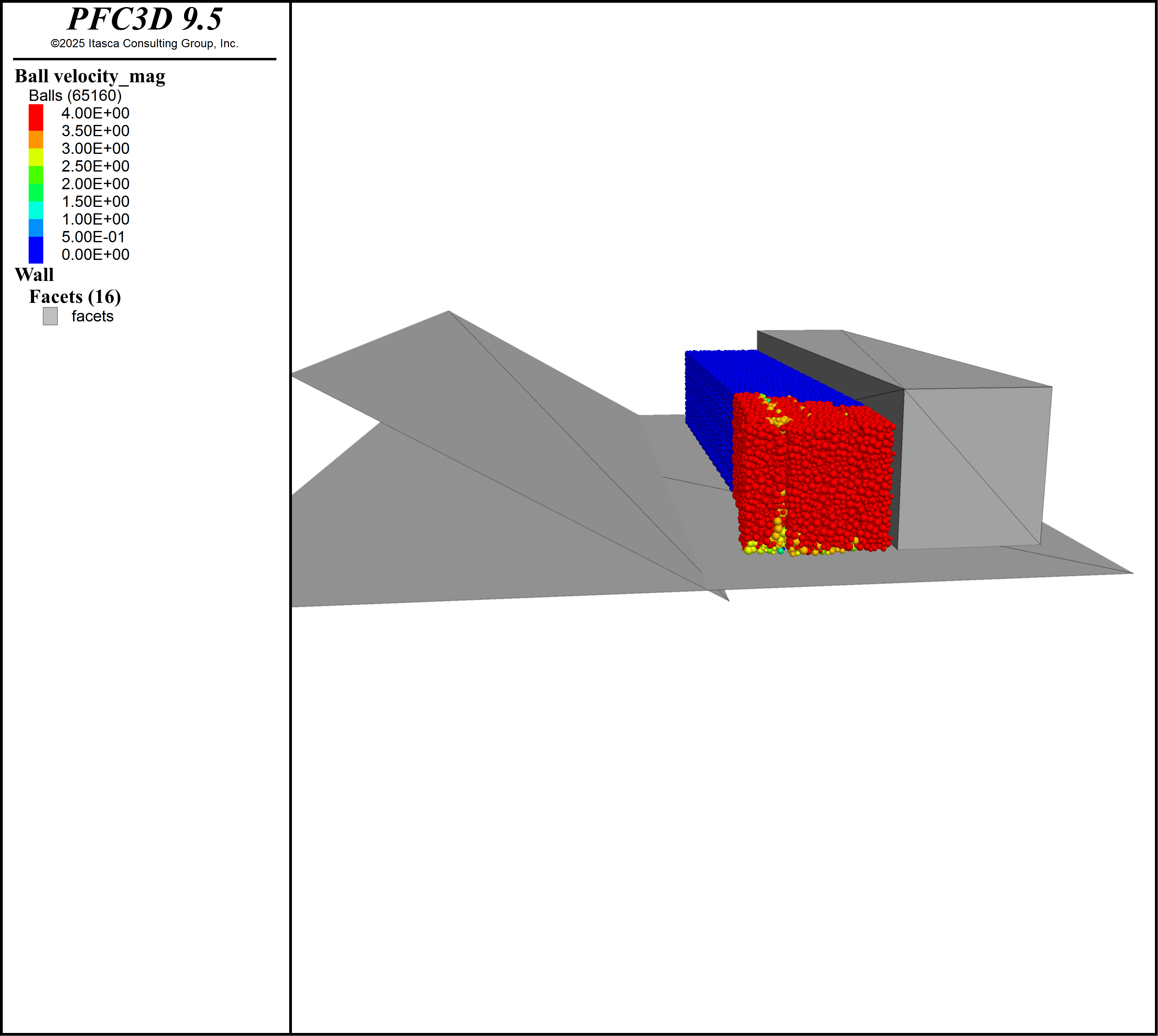
Figure 4: Particles colored by velocity magnitude after 300 ms.
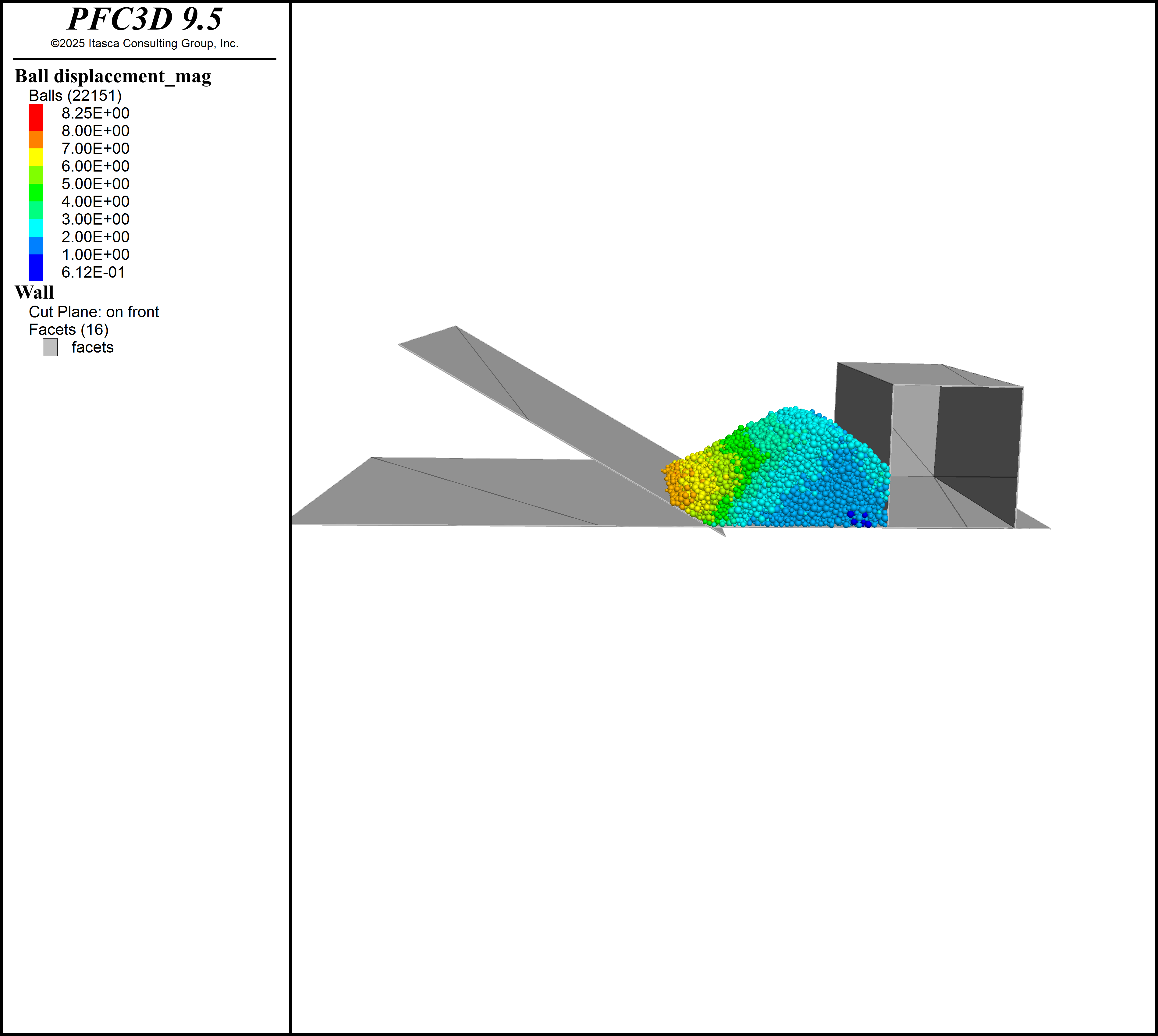
Figure 5: Cross section of the blast muckpile at y=0 showing the particles colored by the distance traveled.
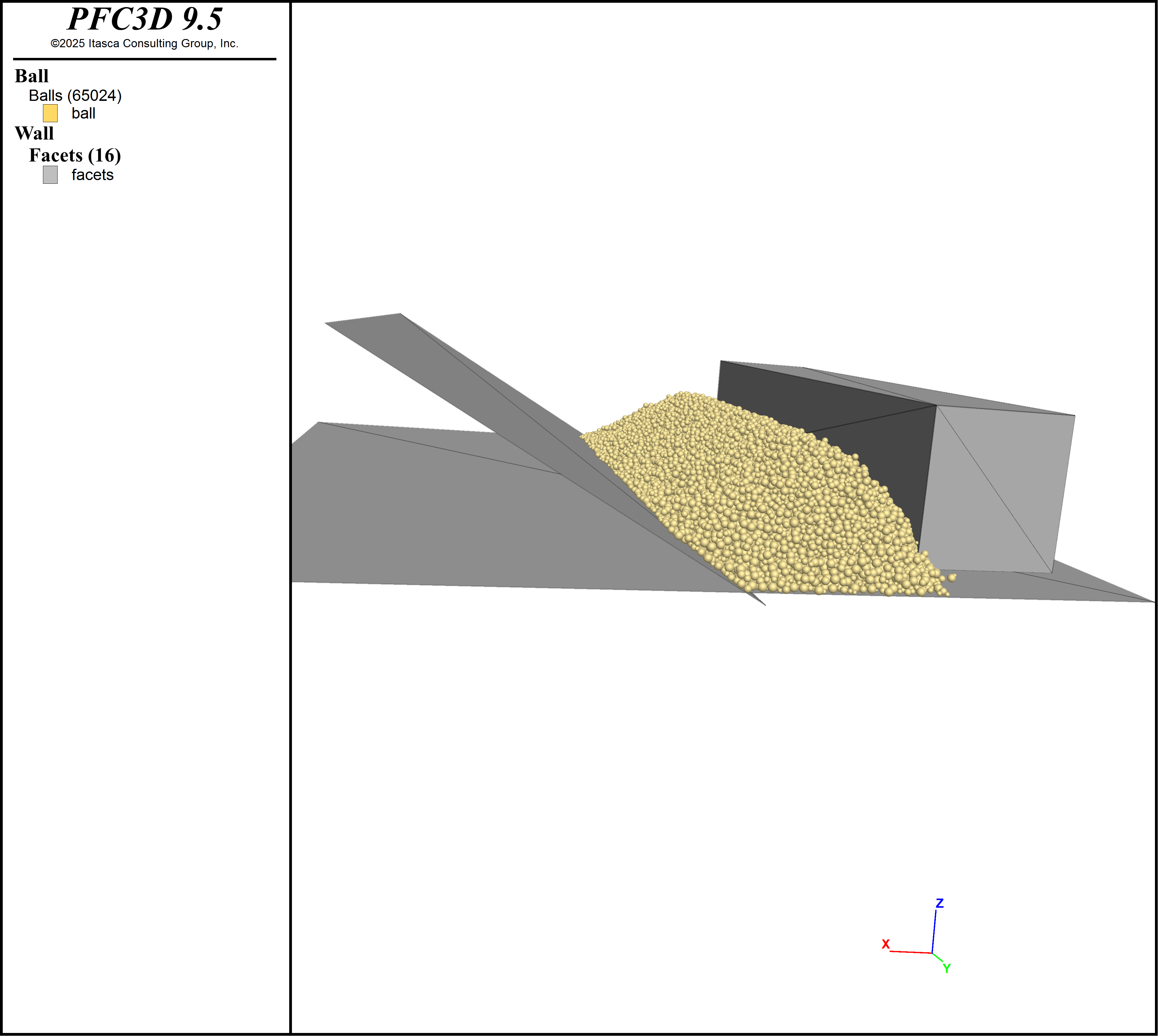
Figure 6: View of the muckpile at the end of the model run.
Data Files
makeBrick.dat
model new
model large-strain true
model random 10000

model domain extent (0, 2) (0, 2) (0, 2) condition periodic

contact cmat default model rrlinear ...
                     property kn 1e6 ks 1e6 fric 0.5 rr_fric 0.0
[global sizeFac = 4.0]
ball distribute box (0 2) (0 2) (0 2) ...
                number-bins 1 ...
                bin 1 radius [sizeFac*0.02] [sizeFac*0.05] volume-fraction 1.0 ...
                porosity 0.4 ; controls number of particles
ball attribute density 1000

ball attribute damp 0.7

model cycle 2000 calm 1
model solve ratio-average 1e-5

measure create id 1 position (0.5,0.5,0.5) radius 0.4
[stressTen = measure.stress( measure.find(1) )]
fish list contents stressTen

brick make id 1
brick export id 1 filename 'myBrick' skip-errors

model save 'myBrick.p3sav'
makeBench.dat
model new
model large-strain on
model title 'Cast Blast - Bench'
model random 10000


[box_x    =  10 ]
[box_y =  10]
[box_z =  3]

; set domain extent and boundary conditions
model domain extent [-1.0*box_x] [3.0*box_x]  ...
              [-2.0*box_y] [3.0*box_y]      ...
              [-.5] [3.0*box_z]         ...
              condition destroy


[dens   =   2.0e3]
[emod   = 1.0e7  ]
[kratio = 2.0    ]
[fric   = 0.5    ]
[dpnr   = 0.2    ]
[dpsr   = 0.2    ]
[dpm    = 3      ]
[rfric  = 0.5    ]

contact cmat proximity 0.1
contact cmat default model rrlinear method deformability    ...
                                       emod        [emod]   ...
                                       kratio      [kratio] ...
                              property fric        [fric]   ...
                                       dp_nratio   [dpnr ]  ...
                                       dp_sratio   [dpsr]   ...
                                       dp_mode     [dpm]    ...
                                       rr_fric     [rfric]


wall generate id 100                ...
              name 'bench'      ...
              box [-0.1*box_x] [0.5*box_x]             ...
                  [-1.5*box_y] [2.5*box_y]             ...
                  0.0 [2*box_z]


brick import id 5 filename 'myBrick'
brick assemble id 5 origin ([-0.4*box_x], [-1.5*box_y], 0) size 5 20 3
ball delete range position-x [0.5*box_x] 1e100
ball delete range position-x -1e100 [-0.1*box_x]
ball attribute damp 0.7

model cycle 1000 calm 10
model solve

contact method deformability emod [emod] kratio [kratio]
contact property fric        [fric]   ...
                                       dp_nratio   [dpnr ]  ...
                                       dp_sratio   [dpsr]   ...
                                       dp_mode     [dpm]    ...
                                       rr_fric     [rfric]
ball attribute density [dens]

contact property lin_mode 1
contact property lin_force (0,0,0)
ball attribute velocity 0
ball attribute spin 0
ball attribute force-contact multiply 0.0 moment-contact multiply 0.0

wall delete

wall generate id 200               ...
              name 'back_bench'      ...
              box [-0.8*box_x] [-0.1*box_x]             ...
                  [-1.5*box_y] [2.5*box_y]             ...
                  0.0 [2.5*box_z]


wall generate id 1               ...
              name 'base_plane'  ...
              plane

wall generate plane dip 30 dip-direction 270 position 8.5 0 0

plot 'Balls' export bitmap filename "blastingthrow_initial.png" size 3800 3400
model save 'bench.sav'
throw_echelon.dat
model restore "bench.sav"
ball attribute damp 0.0
model mechanical time-total 0.0
ball fix velocity
ball fix spin
model gravity 9.81


[XballInitialVelocity = 4.0]
[ZballInitialVelocity = 1]
[timing = 0.05]
[width_blasting = 2]


fish define Timing_Group
    global ncol_=math.ceiling((1.5*box_y + 2.5*box_y)/width_blasting)
    global nrow_=4
    loop n_ (1,ncol_)
        command
            ball group ['Group_'+string(n_)] range position-X [0.35*box_x]  [0.5*box_x] ...
                 position-y [2.5*box_y-width_blasting*(n_)] [2.5*box_y-width_blasting*(n_-1)] ...
                 position-Z  0.0 [2*box_z]
            ball group ['Group_'+string(n_+1)] range position-X [0.2*box_x]  [0.35*box_x] ...
                 position-y [2.5*box_y-width_blasting*(n_)] [2.5*box_y-width_blasting*(n_-1)] ...
                 position-Z  0.0 [2*box_z]
            ball group ['Group_'+string(n_+2)] range position-X [0.05*box_x]  [0.2*box_x] ...
                 position-y [2.5*box_y-width_blasting*(n_)] [2.5*box_y-width_blasting*(n_-1)] ...
                 position-Z  0.0 [2*box_z]
            ball group ['Group_'+string(n_+3)] range position-X [-0.1*box_x]  [0.05*box_x] ...
                 position-y [2.5*box_y-width_blasting*(n_)] [2.5*box_y-width_blasting*(n_-1)] ...
                 position-Z  0.0 [2*box_z]
        endcommand
    endloop
end
[Timing_Group]

program call "set_colors.py"
plot 'Timing' export bitmap filename "blastingthrow_timing.png" size 3800 3400
plot 'StartPosition' export bitmap filename "blastingthrow_startposition.png" size 3800 3400

fish define Cast_Blasting
    loop n_ (1,ncol_+nrow_-1)
        if n_ == 1
          fx = 1
          fy = 0
        else
          fx = Math.sin(Math.deg * 45)
          fy = Math.sin(Math.deg * 45)
        end_if

        command
            ball attribute velocity-x [fx*XballInitialVelocity] ...
                           velocity-y [fy*XballInitialVelocity] ...
                velocity-z [ZballInitialVelocity] range group ['Group_'+string(n_)]
            ball free velocity range group ['Group_'+string(n_)]
            model solve time [timing]
        endcommand
        if n_ = 6
           command
              model save "Echelon_blasting_early.sav"
              plot 'Velocity' export bitmap filename "blastingthrow_velocity.png" size 3800 3400
           end_command
        endif
    endloop
end
[Cast_Blasting]
model solve ratio-average 1e-3
ball attribute damp 0.7
model solve ratio-average 1e-5
model save 'Echelon_blasting_final'
plot 'DistanceTraveled' export bitmap filename "blastingthrow_distancetraveled.png" size 3800 3400
plot 'EndPosition' export bitmap filename "blastingthrow_endposition.png" size 3800 3400
plot 'Balls' export bitmap filename "blastingthrow_final.png" size 3800 3400
python it.fish.set("muck_top", ba.pos()[:,2].max())
Endnote
| Was this helpful? ... | Itasca Software © 2024, Itasca | Updated: Nov 23, 2025 |
