Transient Advection due to Fluid Injection (FLAC2D)

Note

The project file for this example is available to be viewed/run in FLAC2D. The project’s main data files are shown at the end of this example.

Problem Statement

This example considers transient heat transport caused by fluid injection from a well at a constant flow rate. Such processes arise in applications including waste fluid disposal, geothermal energy systems, and subsurface thermal management. A fluid of different temperature is injected into a porous medium through a well, creating a radially outward flow field. As the fluid migrates away from the well, heat is transported primarily by advection, leading to the formation and propagation of a thermal front. The problem is formulated under axisymmetric conditions in FLAC2D, with temperature varying as a function of radial distance and time. The flow field induces a spatially varying velocity that decreases with distance from the well, resulting in non-uniform propagation of the thermal signal with time. This example focuses on the transient evolution of the temperature distribution and the movement of the thermal front under purely advective transport, providing insight into the characteristic behavior of radial convection in porous media systems.

The first step involves establishing a steady-state flow field resulting from constant rate fluid injection, \(Q\), with constant pressure far field. The constant pressure far field is arbitrary as advection responds purely to fluid velocity. In axisymmetric conditions, the radial fluid velocity is given by:

\[v_r \left(r\right) = \frac{Q}{2\pi r h}\]

where \(Q\) is the injection volume flow rate, \(r\) is the radial distance from the well, and \(h\) is the thickness of the porous medium. This velocity field serves as the basis for analyzing the transient thermal response.

The second step involves solving the transient heat transport equation under the established flow field. In the limit of purely advective transport, the governing equation simplifies to:

\[\frac{\partial T}{\partial t} + \eta v_r \frac{\partial T}{\partial r} = 0\]

where \(T\) is temperature, \(t\) is time, \(\eta = \left(\rho C_p\right)_f / \left(\rho C_p\right)_e\) is the ratio of fluid to effective porous media volumetric heat capacity, and \(v_r\) is the radial fluid velocity. This equation describes how the temperature distribution evolves over time due to advection by the flow field. The thermal front propagates outward from the well. Under purely advective conditions, the thermal front position \(r_f\) is:

\[r_f \left(t\right) = \sqrt{r_{w}^2 + \eta \frac{Q}{\pi h} t}\]

The above equation results from the well known solution to the one-dimensional transient advection equation obtained via the method of characteristics, in which the temperature field is binary (either initial temperature or injection temperature) depending on location and time. The analytical solution for thermal front position is programmed as a FISH function and used to compare to numerical results provided by FLAC2D. It is important to note that diffusion is accounted for in FLAC2D, and thus the numerical solution will deviate from the analytical solution, particularly at later times when diffusion causes spreading of the thermal front, e.g., the numerical thermal front will be less sharp.

The following material properties and problem parameters are used in this example:

Geometry:
Well radius (\(r_w\))	0.1 m
Outer radius (\(r_{e}\))	100 m
Thickness of porous medium (\(h\))	1 m
Material Properties:
Density (\(\rho_s\))	2200 kg/m3
Specific heat (\(C_{ps}\))	1000 J/kg-K
Thermal conductivity (\(k_{s}\))	3.0 W/m-K
Fluid density (\(\rho_f\))	1000 kg/m3
Fluid specific heat (\(C_{pf}\))	4200 J/kg-K
Fluid thermal conductivity (\(k_{f}\))	0.6 W/m-K
Porosity (\(n\))	0.2
Initial/Boundary Conditions:
Initial temperature (\(T_0\))	100 C
Injection temperature (\(T_{i}\))	50 C
Injection flow rate (\(Q\))	0.00046 m3/s

This example first establishes the steady-state flow with the command zone fluid steady-state. Second, the transient thermal response is run for 0.25 years, during which the position of the thermal front is tracked with a FISH callback. Note that the numerical thermal front is defined based on the temperature midpoint between injection and initial temperatures which serves as an approximation when diffusion causes spreading over a few meters.

Numerical Stability Considerations

The stability of the numerical solution is governed by the Peclet number, \(P_{e} \leq 2\), and the Courant number, \(C_r \leq 1\), which constrain advective and diffusive transport across each zone. With the fluid velocity field prescribed, the mesh is designed so that the smallest zone near the well satisfies the Peclet stability limit, and zone sizes increase outward at a controlled geometric rate​. The growth rate is selected based on the relative magnitude of diffusion to advection and is capped to prevent excessive zone stretching. The logarithmic term in the calculation of the number of zones arises from summing a geometrically increasing sequence of cell widths needed to span the radius from the well to the external boundary. The mesh parameters for (1) number of zones in the radial direction \(N_{c}\), and (2) the growth rate of the zone size \(g_{c}\) are calculated by the following:

; ------------------------------------------------ ;
; Compute stable mesh size for advection-diffusion
; ------------------------------------------------ ;
fish define MeshParams
    global gc,Nc
    local keff,alpha,beta,dx1,num,den
    ; -------------------------- ;
    keff  = ks*(1-n) + n*kw
    alpha = (4*math.pi*h*keff)/(rhow*cw*Q)
    beta  = 0.8
    ; -------------------------- ;
    dx1   = beta * alpha * Rw
    gc    = math.min(1+alpha,1.05)
    num   = math.ln(1.0 + (Re-Rw)*(gc-1)/dx1)
    den   = math.ln(gc)
    Nc   = math.ceil(num / den)
end
[MeshParams]

Results

The numerical results capture the expected behavior of radial advection under steady-state flow. The radial velocity profile closely matches the analytical solution. The transient temperature field exhibits outward propagation of the thermal front from the injection well. The figure below compares the numerical front position to the purely advective analytical solution, showing good agreement at early times. At later times, diffusion in the numerical model smooths/spreads the front, resulting in a less sharp transition than the analytical prediction. These results illustrate the characteristic spreading of the thermal signal in radial convection through a porous medium.

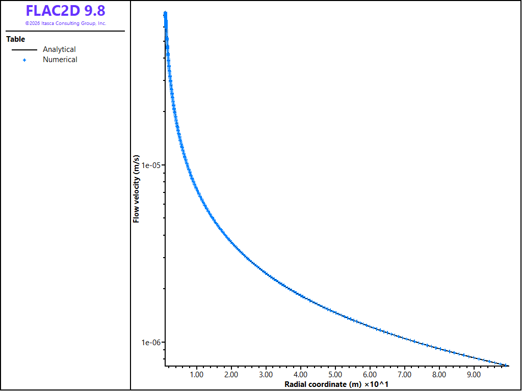
Figure 1: Comparison of analytical and numerical radial velocity profiles under steady-state conditions.

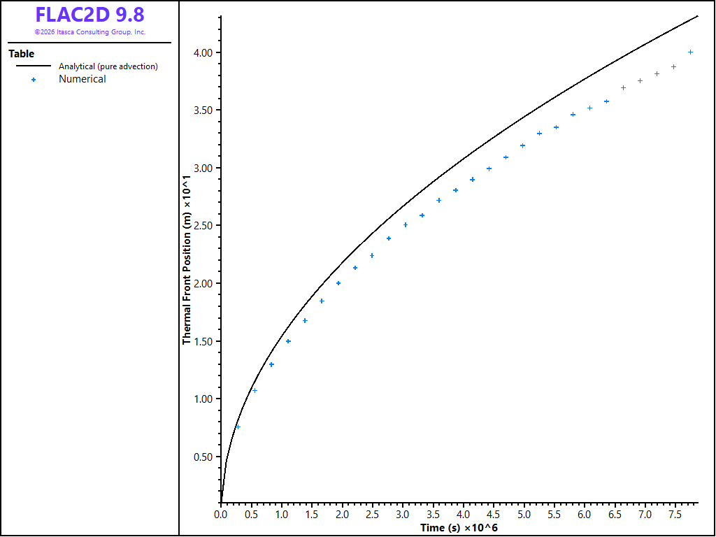
Figure 2: Comparison of numerical thermal font position with time to the purely advective analytical solution.

Data File

radialconvection.dat

model new
model configure fluid-flow thermal
model configure axisymmetry

; Geometry
[Rw = 1.0]      ; Well radius (m)
[Re = 100.0]    ; Outer radius (m)
[h  = 1.0]      ; Height (m)

; Material Properties
[rhos = 2.2e3]  ; Bulk density (kg/(m^3))
[ks = 3.0]      ; Solid conductivity (W/(m*K))
[cs = 1.0e3]    ; Solid specific heat (J/(kg*K))
[n  = 0.2]      ; Porosity (-)

[rhow = 1.0e3]  ; Fluid density (kg/m^3)
[kw = 0.6]      ; Fluid conductivity (W/(m*K))
[cw = 4.2e3]    ; Fluid specific heat (J/(kg*K))

; Initial/Boundary Conditions
[Q  = 4.6e-4]   ; Injection rate (m^3/s)
[T0 = 100.0]    ; Initial temperature (C)
[Tw = 50.0]     ; Injection temperature (C)
[discharge = Q/(2*math.pi*Rw*h)]

program call 'meshparams.dat'

zone create quadrilateral point 0 ([Rw],0) point 1 ([Re],0) ...
    point 2 ([Rw],[h]) point 3 ([Re],[h]) size [Nc] 1 ratio [gc] 1.0
zone face skin

; ---------------------------------------------------- ;
; Step 1: Steady-state flow to initialize flow velocity
; ---------------------------------------------------- ;
zone fluid property porosity [n] mobility-coefficient 1e-10 ...
    fluid-density [rhow]

zone face apply discharge [discharge] range group 'Skin=West'
zone face apply pore-pressure 0.0 range group 'Skin=East'

zone fluid steady-state

; ---------------------------------------------------- ;
; Step 2: Thermal advection for 0.5 year
; ---------------------------------------------------- ;
zone thermal cmodel assign advection-conduction
zone thermal property conductivity-fluid [kw] ...
    specific-heat-fluid [cw] conductivity [ks] ...
    specific-heat [cs]
zone property density [rhos]

zone face apply temperature [Tw] range group 'Skin=West'
zone gridpoint initialize temperature [T0]

program call 'fishhelpers.dat'

fish callback add [track_front] -1 interval 5000
zone thermal timestep fix [dt]
model solve-thermal time-total 7.885e6 ; 0.25 yr