Spherical Cavity with Applied Heat Flux (FLAC2D)

Note

The project file for this example is available to be viewed/run in FLAC2D. The project’s main data files are shown at the end of this example.

Problem Statement

The walls of a spherical cavity in an infinite medium are subjected to a constant heat flux. This problem tests the ability of FLAC2D to perform a transient thermal analysis under spherical axisymmetry conditions. The problem geometry, material properties and initial conditions are defined as:

Geometry:
Sphere radius (\(R\))	0.025 m
Material Properties:
Density (\(\rho\))	2550 kg/m3
Specific heat (\(C_p\))	911.3 J/kg-K
Thermal conductivity (\(k\))	2.51 W/m-K
Initial/Boundary Conditions:
Initial temperature (\(T_0\))	293 K
Applied heat flux (\(q\))	5138.65 W/m2

It is assumed that the material properties are temperature-independent and the flux is constant (no decay). The analytical solution for the transient temperature distribution is given by Carslaw and Jaeger (1959):

\[T(r,t) = \frac{R^2q}{kr} \left[\mathrm{erfc}\left(\frac{r-R}{2\sqrt{\kappa t}}\right) - \mathrm{exp} \left(\frac{r-R}{R} + \frac{\kappa t}{R^2} \right) \mathrm{erfc} \left(\frac{r-R}{2\sqrt{\kappa t}} + \frac{\sqrt{\kappa t}}{R} \right) \right]\]

where \(\kappa\) is the thermal diffusivity, defined as \(\kappa = \frac{k}{\rho C_p}\), \(r\) is the radial coordinate, and \(t\) is time.

A slice of the sphere is modeled by the FLAC2D grid in axisymmetry mode. The command zone create sector-quad is used to create the grid. The heat flux is applied to the wall of the sphere; all other boundaries of the grid are adiabatic. The adiabatic boundary is correct for the lines of symmetry at \(x=0\) and \(y=0\). The outer boundaries are located 0.25 m from the symmetry lines (10 times the sphere radius); the adiabatic condition there does not influence the results for the selected heating duration (5000 seconds).

Results

The results for temperature distribution and comparison of analytical and numerical solutions are shown in the following figures. Analytical and numerical temperature solutions are compared at three locations; radial distances of 0.025 m, 0.038 m, and 0.055 m from the center of the sphere. The difference between analytical and numerical temperatures at these locations is less than 1% at 5000 seconds.

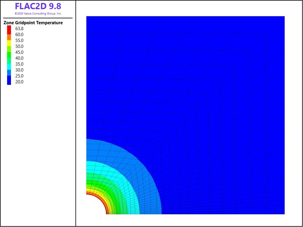
Figure 1: Temperature distribution at 5000 seconds.

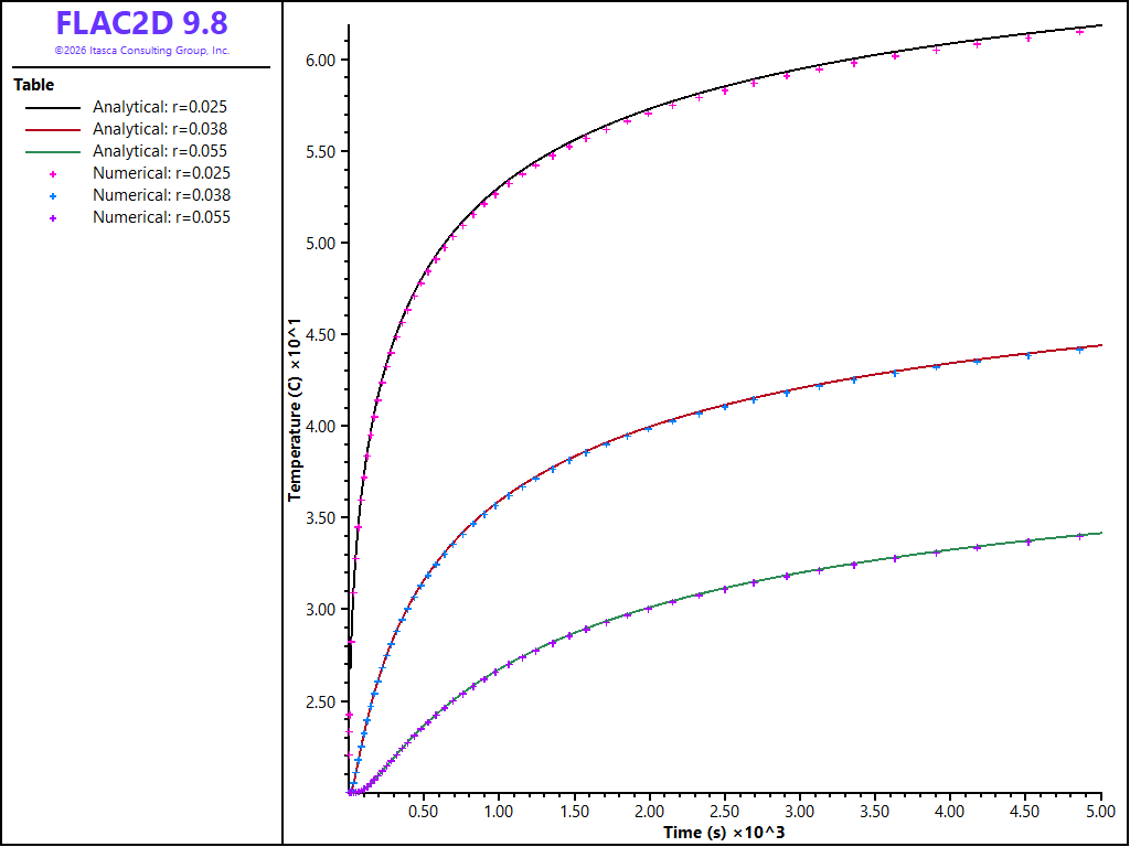
Figure 2: Comparison of analytical and numerical temperature solutions at three locations.

Reference

Carslaw, H. S. and Jaeger, J. C. Conduction of Heat in Solids, 2nd ed., Oxford University Press, New York (1959).

Data File

sphericalcavityheatflux.dat

model new
model configure axisymmetry thermal

[R = 0.025]     ; Sphere radius (m)
[q = 5138.64]   ; Applied heat flux (W/m^2)
[k = 2.51]      ; Thermal conductivity (W/(m*K)
[c = 911.3]     ; Heat capacity (J/(kg*K)
[rho = 2550]    ; Density (kg/(m^3))

zone create sector-quad point 0 (0,0) point 1 ([10*R],0) ...
    point 2 (0,[10*R]) point 3 ([10*R],[10*R]) point 4 ([R],0) ...
    point 5 (0,[R]) size 1 25 25 ratio 1.0 1.1 1.1
zone face skin

zone thermal property conductivity [k] specific-heat [c]
zone property density [rho]

zone gridpoint initialize temperature 20

zone face apply flux [q] range group 'Skin=West1'

history interval 25
model history name 't' thermal time-total
zone history name '2.5_' temperature position (0.025,0.0)
zone history name '3.8_' temperature position (0.038,0.0)
zone history name '5.5_' temperature position (0.055,0.0)

model solve-thermal time-total 5000