Seismic Analysis of an Embankment Dam (FLAC2D)
Problem Statement
The project file for this example may be viewed/run in FLAC2D.[1] The main data files used are shown at the end of this example.
An analysis of the seismic performance of an embankment dam should consider static-equilibrium and coupled groundwater conditions, as well as fully dynamic processes. This includes calculations for (1) the state of stress prior to seismic loading, (2) the reservoir elevation and groundwater conditions, (3) the mechanical behavior of the foundation and embankment soils including the potential for liquefaction, and (4) the site-specific ground motion response. This example presents a FLAC2D model for an embankment dam that demonstrates a procedure to incorporate these processes and calculations in the seismic analysis.
The example is a simplified representation of a typical embankment dam geometry. The dam is 130 ft high and 1120 ft long. It is constructed above a layered foundation of sandstone and shale materials. The crest of the dam is at elevation 680 ft when the seismic loading is applied. The embankment materials consist of a low-permeability, clayey-sand core zone with upstream and downstream shells of gravelly, clayey sands. These soils are considered to be susceptible to liquefaction during a seismic event. The materials in this analysis are defined as foundation soils 1 and 2 and embankment soils 1 and 2, as depicted in Figure 1.
The earth dam is subjected to seismic loading representative of the 1987 Loma Prieta earthquake in California. The earthquake target motion for this model is taken from that recorded at the left abutment of the Lexington Dam during the Loma Prieta earthquake and, for this analysis, the input is magnified somewhat and assumed to correspond to the acceleration at the surface of the foundation soils at elevation 550 ft. The target record is provided in the file named “ACC_TARGET.ACC.” The estimated peak acceleration is approximately 12 ft/sec2 (or 0.37 g), and the duration is approximately 40 sec. The record is shown in Figure 2.

Figure 1: Embankment dam.
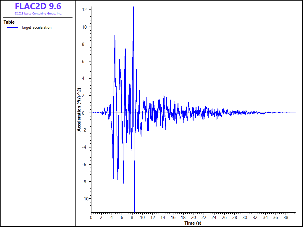
Figure 2: Horizontal acceleration at elevation 550 ft – target motion.
Modeling Procedure
This example illustrates a recommended procedure to simulate seismic loading of an embankment dam with FLAC2D. A coupled effective-stress analysis is performed using a “simple” material model to simulate the behavior of the soils, including liquefaction. The soil behavior is based upon the Mohr-Coulomb plasticity model with material damping added to account for cyclic dissipation during the elastic part of the response and during wave propagation through the site. Liquefaction is simulated by using the Finn-Byrne model, which incorporates the Byrne (1991) relation between irrecoverable volume change and cyclic shear-strain amplitude into the Mohr-Coulomb model.
The modeling procedure is divided into seven steps.
Waveform processing.
Model setup.
Assign material properties.
Calculate the static equilibrium state for the site including the steady-state groundwater conditions with the reservoir at full pool.
Apply the dynamic loading conditions.
Perform preliminary elastic undamped simulations to check model conditions.
Run a simulation with actual strength properties and representative damping, assuming the soils do not liquefy in order to evaluate the model response.
Perform the seismic calculation assuming the soils can liquefy.
These steps are described separately in the sections below.
Waveform processing
An acceleration history from the 1987 Loma Prieta earthquake recorded at the surface is provided in FLAC2D table format in the file acc_target.acc. This can be imported and plotted using the table import command as shown in Figure 2.
To get the waveform for input at the base of the model, a deconvolution is required. The appropriate input motion at depth is computed by performing a deconvolution analysis using the equivalent-linear program SHAKE. This approach is reasonable, provided the model exhibits a low level of nonlinearity. SHAKE-91 (Idriss and Sun 1992) is used in this example to estimate the appropriate motion at depth corresponding to the target (surface) motion. This deconvoluted motion should then produce the target motion at the surface. In this example, the upward-propagating motion calculated from SHAKE-91 is used with a compliant-base boundary. Note that SHAKE-91 accelerations are in g’s versus seconds, and need to be converted into ft/sec2 versus seconds when applied in FLAC2D. The input record (i.e., the upward-propagating motion from the deconvolution analysis and converted to ft/sec2) is in the file named “ACC DECONV.HIS,” (also in table format) and is shown in Figure 3. The peak acceleration is roughly half of the peak acceleration at the surface—the doubling effect that occurs at the free surface has been mostly removed by the deconvolution.
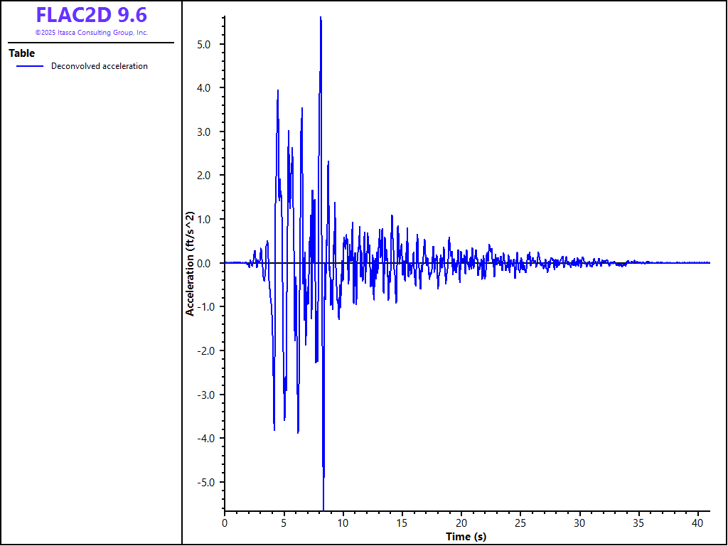
Figure 3: Horizontal acceleration at base of model (elevation = 400 feet).
The waveform then requires further processing for use in FLAC2D. To ensure accurate propagation of the waves, there should be at least 10 zones per wavelength. It is therefore necessary to filter out high frequencies (after first checking that not much energy is contained in the high frequencies). It is also necessary to do a baseline correction so there is not a permanent displacement at the bottom. Finally, the wave is saved as a velocity instead of an acceleration for application as a boundary condition in FLAC2D. These steps are performed with the Dynamic Input Wizard and are described here: Dynamic Input Wizard. The resulting input wave is saved to the file table104.dat included with this project and shown in Figure 9.
Model setup
The model is created in Sketch by following these steps.
Create a rectangle from (0,400) to (1800,550).
Draw a horizontal line at y=475.
Draw a polyline to define the dam trough these points: (350,550) (720,680) (800,680) (1470,550).
Draw lines to define the core of the dam: (628,550) to (720,680) and (900,550) to (800,680).
Set the number of zones across the extent to 180, ensure that only unstructured meshes are being created and zoned the model.
Set the group names as shown in Figure 1.
Generate the zones and save the model.
Material Properties
The foundation and embankment soils are modeled as Mohr-Coulomb materials. Drained properties are required because this is an effective-stress analysis. The properties for the different soil types are listed in Table 1.
Property |
Foundation Soil 1 |
Foundation Soil 1 |
Embankment Soil 1 |
Embankment Soil 2 |
|---|---|---|---|---|
Unit weight (pcf) |
125 |
125 |
113 |
120 |
Young’s modulus (ksf) |
12757 |
12757 |
6838 |
6838 |
Poisson’s ratio |
0.3 |
0.3 |
0.3 |
0.3 |
Cohesion (psf) |
83.5 |
160 |
120 |
120 |
Friction angle (degrees) |
40 |
40 |
35 |
35 |
Dilation angle (degrees) |
0 |
0 |
0 |
0 |
Porosity |
0.3 |
0.3 |
0.3 |
0.3 |
Hydraulic conductivity (ft/s) |
3.3 × 10⁻⁶ |
3.3 × 10⁻⁷ |
3.3 × 10⁻⁶ |
3.3 × 10⁻⁸ |
Establish Initial State of Stress
This model requires configuring fluid and dynamic analysis (model configure fluid-flow dynamic). For this stage, both fluid and dynamic are off. This model follows the standard boundary conditions: fixed degrees of freedom at the bottom and roller boundaries on the sides.
State of Stress before Raising Reservoir Level
The analysis is started from the state before the embankment is constructed. The construction process may affect the stress state, particularly if excess pore pressures develop in the soils and do not dissipate completely during the construction stages. The embankment can be constructed in stages, with a consolidation time specified in the FLAC2D model, if pore-pressure dissipation is a concern. In this example, the excess pore pressures are assumed to dissipate before a new lift of embankment material is placed.
It should be noted that staged modeling of the embankment lift construction also provides a better representation of the initial, static shear stresses in the embankment. This is important, particularly in a liquefaction analysis, because the initial, static shear stresses can affect the triggering of liquefaction. In this simplified example, the embankment is placed in one stage. However, it is recommended that the lift construction stages be simulated as closely as is practical, in order to provide a realistic representation of the initial stress state.
The embankment materials are temporarily removed from the model. These materials will be added back after the calculation for the initial equilibrium state of the foundation.
zone null range group 'embankment:soil_1'
zone null range group 'embankment:soil_2'
An initial stress state given by a coefficient of earth pressure at rest of 0.5 is assumed. The water table is located at elevation 550 ft. Pore pressure changes due to deformation (undrained effect) are inhibited using the command zone fluid property pore-pressure-generation off.
The model is cycled to equilibrium by the command:
model solve-static elastic convergence 1
Figure 4 shows the initial pore-pressure distribution in the foundation soils.
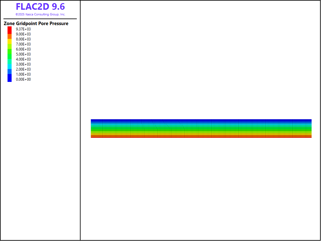
Figure 4: Pore pressure distribution in foundation soils.
To simulate the construction process the embankment materials can be added to the model in stages using the commands:
zone cmodel assign mohr-coulomb range group 'embankment:soil_2'
zone property density 3.73 young 6838e3 poisson 0.3 cohesion 120.0 ...
              friction 35.0 dilation 0.0 tension 0.0 ...
              range group 'embankment:soil_2'
zone cmodel assign mohr-coulomb range group 'embankment:soil_1'
zone property density 3.51 young 6838e3 poisson 0.3 cohesion 120.0 ...
In this example, both embankment soils 1 and 2 are added simultaneously, and pore pressures are assumed not to change. The displacements resulting from adding the embankment in one step are shown in Figure 5. This “construction step” is done to simplify the example; a more rigorous analysis should follow the construction sequence as closely as possible, in order to produce a more realistic displacement pattern and initial stress state.
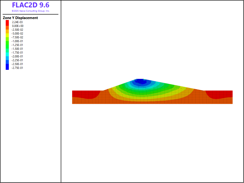
Figure 5: Displacements induced by embankment construction in one step.
State of Stress with the Reservoir Level Raised
The earthquake motion is considered to occur when the reservoir level is at full pool (i.e., at its full height at elevation 670 ft). For this stage of the analysis, the pore-pressure distribution through the embankment and foundation soils is calculated for the reservoir raised to this height. The following command is used to set the pore-pressure distribution on the upstream side of the embankment:
zone face apply head 670 ...
           range group 'West' or 'Top' position-y 400 670 position-x 0 693
The pore pressures are fixed at gridpoints along the downstream slope to allow flow across this surface. The steady state pore pressures are then calculated with the command zone fluid-steady-state. Note that the steady state solution does not converge for the default error tolerance, so the tolerance is relaxed slightly from 1e-4 (the default) to 1e-3.
Figure 6 displays the pore-pressure distribution through the embankment and foundation at steady state.
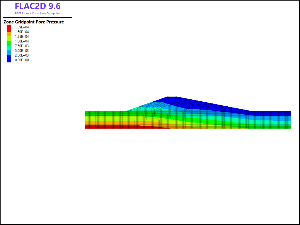
Figure 6: Pore-pressure distribution at steady state flow for reservoir raised to 670 ft.
The static equilibrium state is now calculated for the new pore-pressure distribution. A pressure distribution is applied along the upstream slope to represent the weight of the reservoir water. The model is now solved for this applied condition, and the resulting total vertical-stress contour plot for the model at this stage is shown in Figure 7.
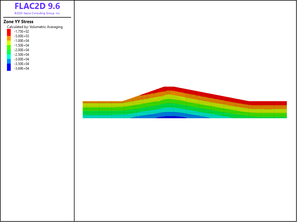
Figure 7: Total vertical-stress distribution at steady state flow for reservoir raised to 670 ft.
Factor of Safety for Embankment Dam
This is considered to be the state of the embankment dam at the time of the earthquake event. A factor-of-safety calculation (model factor-of-safety) is done as a check on the stability condition at this state. The result, plotted in Figure 8, shows that the safety factor is 2.43 and the weakest failure surface develops along the upstream slope.

Figure 8: Factor-of-safety plot for embankment dam at full pool.
Apply Dynamic Loading Conditions
For the dynamic loading stage, pore pressures can change in the materials due to dynamic volume changes induced by the seismic excitation. In order for pore pressures to change as a result of volume change, the actual value of water bulk modulus must be prescribed. For this scenario, it was estimated that the fluid bulk modulus was 4.1 × 10⁶ psf (presumably the water contained some dissolved air, since the usual bulk modulus of fluid at room temperature is about 4.6 × 10⁷ psf).
Note
For these “undrained” analyses, it may be assumed that a fluid stiffness of more than about 20× the soil stiffness can be considered essentially infinite (incompressible). The command zone fluid modulus-automatic could be added after setting the true fluid modulus. This will automatically reduce the fluid stiffness if it is significantly more stiff than the soil in order the increase the calculated dynamic timestep. In this model it is not necessary since the specified fluid bulk modulus is already less than this “incompressible” value.
Note that the groundwater-flow mode is not active, because it is assumed that the dynamic excitation occurs over a much smaller time frame than required for pore pressures to dissipate.
The dynamic calculation mode and large-strain mode are turned on. The model should be re-initialized to zero displacements and velocities: in this way, only seismic induced motions and deformations are shown in the model results.
The dynamic boundary conditions are now applied. In this model, a compliant boundary condition is assumed for the base (i.e., the foundation materials are assumed to extend to a significant depth beneath the dam). Therefore, it is necessary to apply a quiet (viscous) boundary along the bottom of the model to minimize the effect of reflected waves at the bottom. The filtered and baseline-corrected input velocity is stored in table 104. The input velocity motion is then converted into a shear stress history. The free-field boundary is set for the side boundaries. The commands are:
program call 'mon_ex.fis'
zone property cohesion 1e20 tension 1e20
[global mf = -2*4.462*1048.6] ;cs=1048.6, density=4.462
zone face apply stress-xy [mf] table 'tab104' range group 'Bottom'
Run Undamped Dynamic Simulations
Before running a dynamic model with actual material strength and damping properties, preliminary runs are performed to assess the effect of model boundary locations, and to estimate the maximum levels of cyclic strain and natural frequency ranges of the model system. These runs also help to evaluate the necessity for additional material damping in the model.
The input velocity applied at the base of the model is checked first to ensure that the calculated velocity corresponds to the input velocity. The bottom boundary is deep enough so that velocity doubling has only a small effect on the calculated velocity at the model base. The comparison of calculated velocity to input velocity is shown in Figure 9. There is a slight difference between the input and calculated velocity.
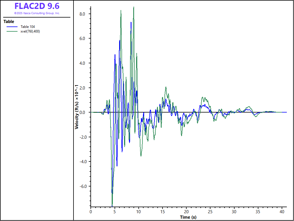
Figure 9: Comparison of velocity histories at the base and top of model of undamped elastic material.
Run Damped Simulations with Actual Mohr-Coulomb Strength Properties
Hysteretic damping is applied to the model. The selected parameters (L1 = −3.156 and L2 = 1.904) for the default model are used. These values are obtained from curve fitting to data for clay (see Hysteretic Damping). Hysteretic damping does not completely damp high-frequency components, so a small amount of stiffness-proportional Rayleigh damping is also applied. A value of 0.2% at the dominant frequency (1.0 Hz) is assigned.
The dynamic boundary conditions are applied in the same way as for the undamped elastic simulation.
Movement of the embankment after 40 seconds is primarily concentrated along the upstream slope. This is shown in the \(x\)-displacement contour plot Figure Figure #xdisp-MC and the shear-strain increment contour plot Figure Figure #shear-strain-MC. The movement recorded at (606,640) along the upstream slope is shown in Figure Figure #rel-disp-MC. The effect of material failure and hysteretic damping is evident in the cyclic shear strain response.
The pore pressure and effective vertical stress histories in Figure Figure #pp-esyy-MC, recorded at (471,558) near the upstream face, illustrate the minor pore-pressure change in the embankment materials during the seismic loading.
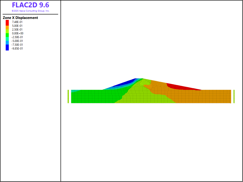
Figure 10: \(x\)-displacement contours at 40 seconds – Mohr-Coulomb material and hysteretic damping.
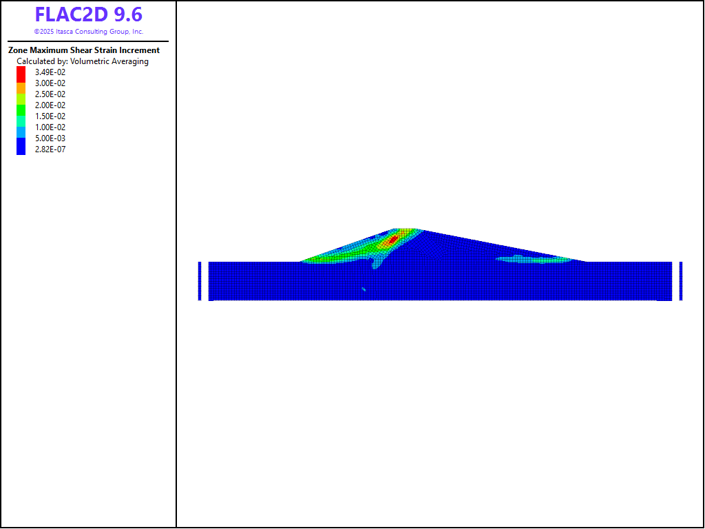
Figure 11: Shear-strain increment contours at 40 seconds – Mohr-Coulomb material and hysteretic damping.
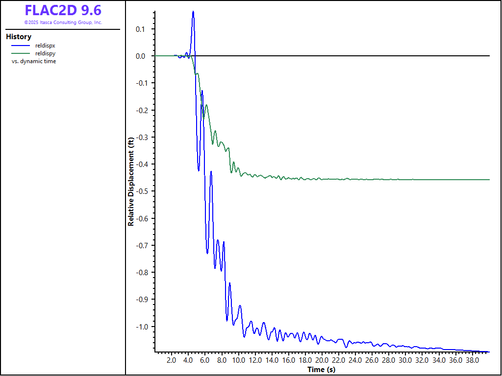
Figure 12: Relative displacements along upstream slope– Mohr-Coulomb material and hysteretic damping.
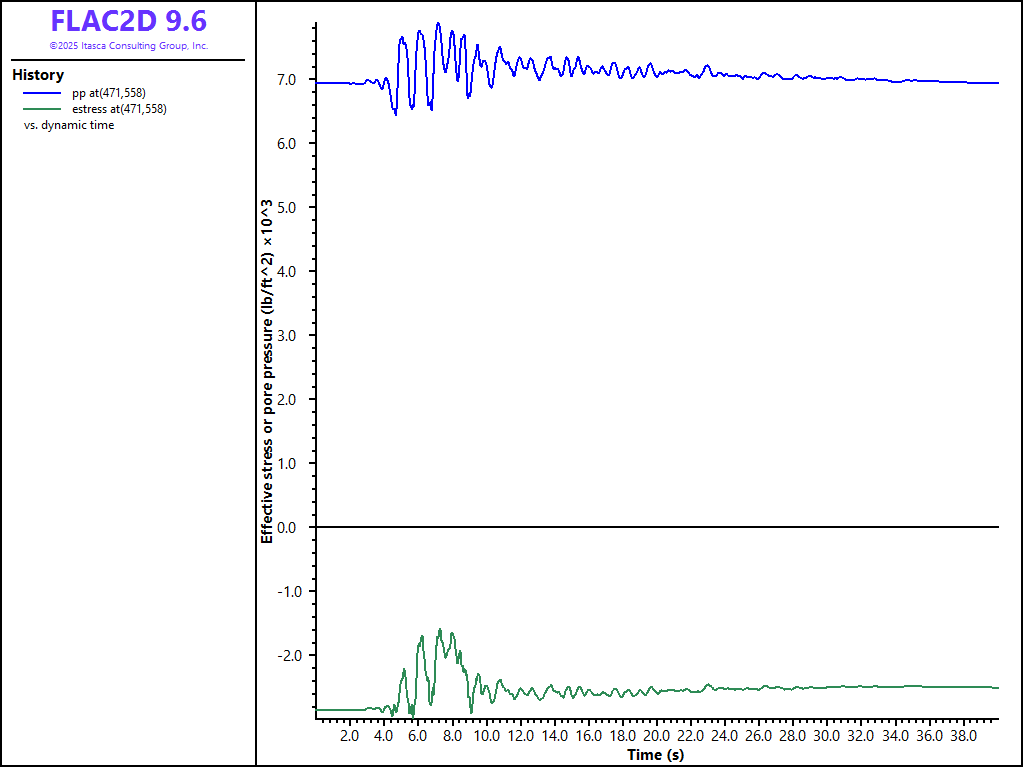
Figure 13: Pore-pressure and effective vertical stress near upstream slope – Mohr-Coulomb material and hysteretic damping.
Run Seismic Calculation Assuming Liquefaction
The embankment soils are now changed to liquefiable materials. The Finn-Byrne liquefaction model is prescribed for embankment soils 1 and 2, with parameters set to correspond to SPT measurements. For a normalized SPT blow count of 10, the Byrne model parameters are C1 = 0.2452 and C2 = 0.8156. The value for latency is set to 1,000,000 at this stage. This is done to prevent the liquefaction calculation from being activated initially. The model is first checked to make sure that it is still at an equilibrium state when switching materials to the Byrne model, before commencing the dynamic simulation.
The model is now ready for the dynamic analysis. The water bulk modulus is assigned as 4.6 × 10⁷ psf (and scaled). The value for latency of the embankment soils is reduced to 50. The dynamic conditions are now set again in the same manner as described above. Change in pore pressure, or excess pore pressure, is calculated throughout the model in order to evaluate the potential for liquefaction. The normalized excess pore-pressure ratio can be used to identify the region of liquefaction in the model. (The excess pore-pressure ratio is calculated in FISH function “GETEXCESSPP.FIS”.)
The model is now run for a dynamic time of 40 seconds. The results in the figures below show the effect of pore-pressure generation in the embankment soils. There is now a substantial movement along the upstream face, as seen in the figures. The relative vertical settlement at (606,640) is now approximately 1.2 ft, and the relative shift upstream is approximately 3.4 ft, as shown in Figure 16. A significant increase in pore pressure (and decrease in effective stress) is calculated in the upstream region, as indicated in Figure 17. The location of the pore pressure/effective stress measurement is at (471,558), which is at a depth of approximately 35 ft below the upstream slope face, and 115 ft from the toe of the upstream slope. Contours of the cyclic pore-pressure ratio greater than 0.99 are plotted in Figure 18. These contours show the extent of the liquefied embankment soils, primarily in the upstream region.
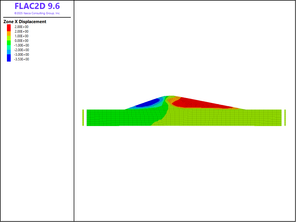
Figure 14: \(x\)-displacement contours at 40 seconds – Byrne (liquefaction) material and hysteretic damping.
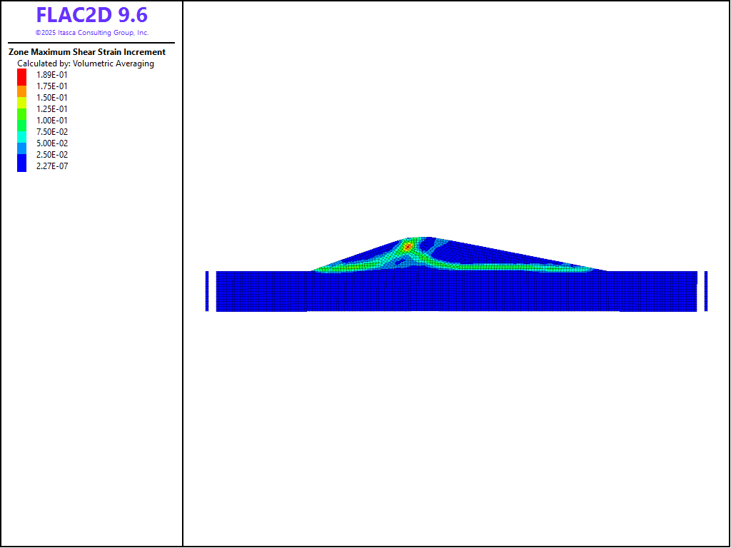
Figure 15: Shear-strain increment contours at 40 seconds – Byrne (liquefaction) material and hysteretic damping.
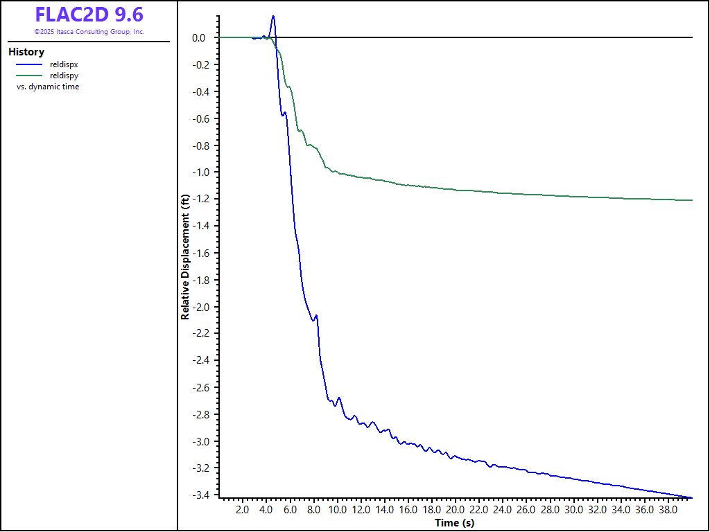
Figure 16: Relative displacements along upstream slope – Byrne (liquefaction) material and hysteretic damping.
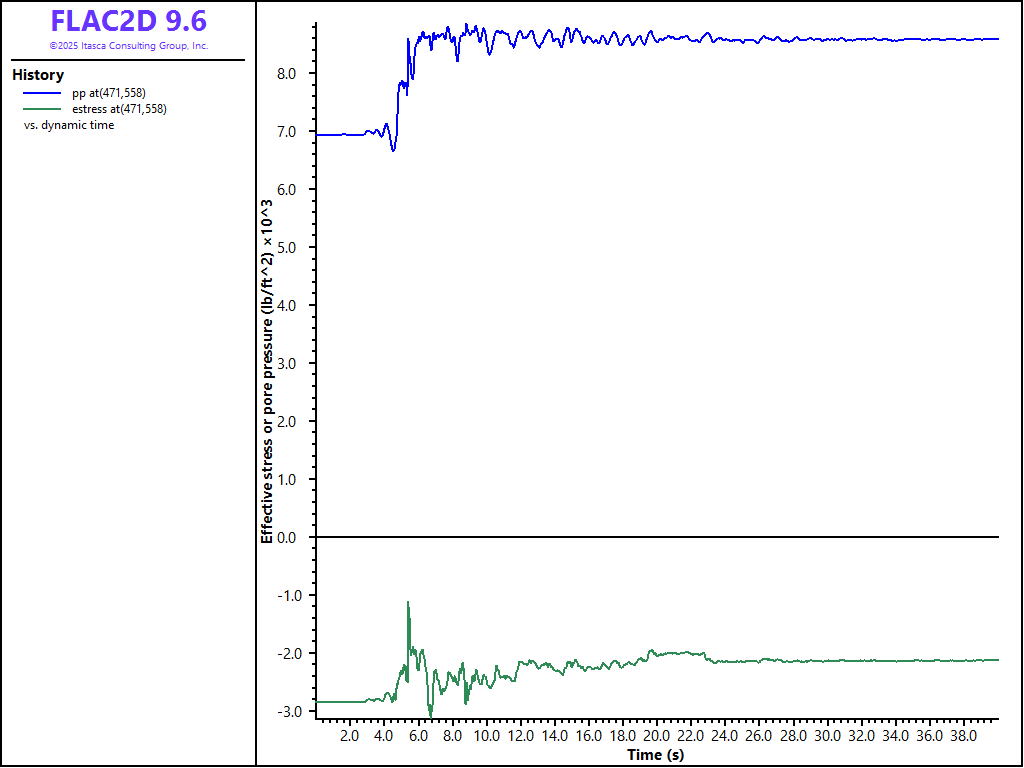
Figure 17: Pore-pressure and effective vertical stress near upstream slope– Byrne (liquefaction) material and hysteretic damping.
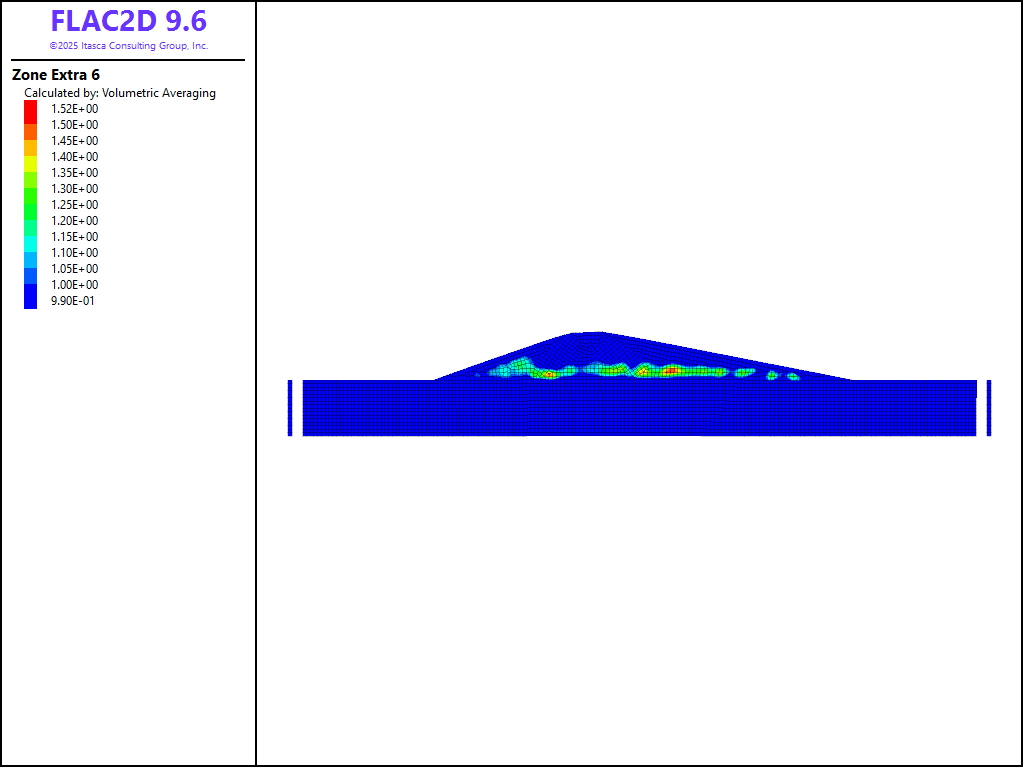
Figure 18: Excess pore-pressure ratio (values greater than 0.99) – Byrne (liquefaction) material and Rayleigh damping.
Acknowledgment
This example is derived from data provided by Dr. Nason McCullough of CH2MHill. His assistance and critical review of this exercise are gratefully acknowledged.
References
Byrne, P. M. “A Cyclic Shear-Volume Coupling and Pore-Pressure Model for Sand,” in Proceedings: Second International Conference on Recent Advances in Geotechnical Earthquake Engineering and Soil Dynamics (St. Louis, Missouri, March 1991), Paper No. 1.24, 47-55 (1991).
Idriss, I. M., and Joseph I. Sun. User’s Manual for SHAKE-91. University of California, Davis, Center for Geotechnical Modeling, Department of Civil & Environmental Engineering (November 1992).
Data Files
edam_assign_props.dat
model new
program call 'sketch'
model configure fluid-flow dynamic
model gravity 32.2
model large-strain off

zone cmodel assign mohr-coulomb
zone face skin

zone property density=[125/32.2] young 12757e3 poisson 0.3 cohesion=83.5 ...
     friction=40.0 dilation=0.0 tension=0.0 range group 'foundation:soil_1'

zone property density [125/32.2] young 12757e3 poisson 0.3 cohesion 160.0 ...
     friction 40.0 dilation 0.0 tension 0.0 range group 'foundation:soil_2'

zone property density=[113/32.2] young 6838e3 poisson 0.3 cohesion=120.0 ...
     friction=35.0 dilation=0.0 tension=0.0  range group 'embankment:soil_1'

zone property density=[120/32.2] young 6838e3 poisson 0.3 cohesion=120.0 ...
     friction=35.0 dilation=0.0 tension=0.0 range group 'embankment:soil_2'

zone fluid property porosity 0.3
zone fluid property hydraulic-conductivity 3.3E-6 ...
                    range group 'foundation:soil_1'
zone fluid property hydraulic-conductivity 3.3E-7 ...
                    range group 'foundation:soil_2'
zone fluid property hydraulic-conductivity 3.3E-6 ...
                    range group 'embankment:soil_1'
zone fluid property hydraulic-conductivity 3.3E-8 ...
                    range group 'embankment:soil_2'
model save 'edam_assign_props'
edam_initial.dat
model restore 'edam_assign_props'
zone null range group 'embankment:soil_1'
zone null range group 'embankment:soil_2'

; Boundary conditions - roller on sides, fixed on bottom
zone face apply velocity-x 0 range group 'East' or 'West'
zone face apply velocity (0,0) range group 'Bottom'

zone fluid density 1.94
zone fluid unsaturated cutoff
zone fluid property pore-pressure-generation off
zone gridpoint pore-pressure head 550
zone initialize-stresses ratio 0.5

model history name 'unbal' mechanical ratio-maximum
model solve-static elastic convergence 1
model save 'edam_initial'
edam_add_embank.dat
model restore 'edam_initial'
zone fluid property pore-pressure-generation off
zone cmodel assign mohr-coulomb range group 'embankment:soil_2'
zone property density 3.73 young 6838e3 poisson 0.3 cohesion 120.0 ...
              friction 35.0 dilation 0.0 tension 0.0 ...
              range group 'embankment:soil_2'
zone cmodel assign mohr-coulomb range group 'embankment:soil_1'
zone property density 3.51 young 6838e3 poisson 0.3 cohesion 120.0 ...
              friction 35.0 dilation 0.0 tension 0.0 ...
              range group 'embankment:soil_1'
model solve-static convergence 1
model save 'edam_add_embank'
edam_fluid_flow.dat
model restore 'edam_add_embank'
;zone fluid property pore-pressure-generation on
zone face apply head 670 ...
           range group 'West' or 'Top' position-y 400 670 position-x 0 693
zone gridpoint fix pore-pressure range group 'Top' position-x 800 1800

; reach new steady-state fluid flow
zone fluid unsaturated cutoff
zone fluid steady-state tolerance 1e-3

model save 'edam_fluid_flow.sav'
edam_static.dat
model restore 'edam_fluid_flow'
zone face apply stress-normal [-670*1.94*32.2] gradient 0 [1.94*32.2] ...
           range group 'Top' position-y 550 670 position-x 0 693

model solve-static convergence 1
model save 'edam_static'

zone gridpoint initialize displacement (0,0)
zone gridpoint initialize velocity (0,0)

model dynamic active off
model fluid active off
model factor-of-safety
model save 'edamfos.sav'
edam_dyn_elastic.dat
model restore 'edam_static'
model large-strain on
model dynamic active on
model fluid active off
zone fluid property fluid-modulus 4.1e6
zone fluid property pore-pressure-generation on

zone gridpoint initialize displacement (0,0)
zone gridpoint initialize velocity (0,0)
zone initialize state 0
table 'tab104' import "table104.dat"

program call 'strain_hist.fis'
program call 'reldispx.fis'
program call 'excpp.fis'

model history name 'dynamic time' dynamic time-total
zone history name 'shear stress' stress quantity xy position (760,595)
fish history name 'shear strain' str_77_20
fish history name 'reldispx'  reldispx
fish history name 'reldispy' reldispy
fish history name 'excess pp' excpp
zone history name 'pp at(471,558)' pore-pressure position (471,558)
zone history name 'estress at(471,558)' ...
                   stress-effective quantity yy position (471,558)
zone history name 'xacc at(760,400)' acceleration-x position (760,400)
zone history name 'xacc at(753,679)' acceleration-x position (753,679)
zone history name 'xacc at(1708.5,549.8)' ...
                   acceleration-x position (1708.5,549.8)
zone history name 'xacc at(82,549.8)' acceleration-x position (82,549.8)
zone history name 'xvel at(760,400)' velocity-x position (760,400)
zone history name 'xvel at(753,679)' velocity-x position (753,679)
zone history name 'xvel at(1708.5,549.8)' velocity-x position (1708.5,549.8)
zone history name 'xvel at(82,549.8)' velocity-x position (82,549.8)
zone history name 'xvel at(756,570.5)' velocity-x position (756,570.5)
zone history name 'strain inc at(755,590)' strain-increment position (755,590)
history interval 100

program call 'mon_ex.fis'
zone property cohesion 1e20 tension 1e20
[global mf = -2*4.462*1048.6] ;cs=1048.6, density=4.462
zone face apply stress-xy [mf] table 'tab104' range group 'Bottom'
zone face apply quiet range group 'Bottom'
zone dynamic free-field on
zone nodal-mixed-discretization off
model solve-dynamic time-total 40
history export 'xvel at(760,400)' vs 'dynamic time' table 'xvel(760,400)'
model save 'edam_dyn_elastic.sav'
edam_dyn_MC.dat
model restore 'edam_static'
zone fluid property fluid-modulus 4.1e6
zone fluid property pore-pressure-generation on
model large-strain on
model dynamic active on
model fluid active off
zone gridpoint initialize displacement (0,0)
zone gridpoint initialize velocity (0,0)
zone initialize state 0
table 'tab104' import "table104.dat"

program call 'strain_hist.fis'
program call 'reldispx.fis'
program call 'excpp.fis'

model history name 'dynamic time' dynamic time-total
fish history name 'shear strain' str_77_20
fish history name 'reldispx'  reldispx
fish history name 'reldispy' reldispy
fish history name 'excess pp' excpp
zone history name 'pp at(471,558)' pore-pressure position (471,558)
zone history name 'estress at(471,558)' ...
                   stress-effective quantity yy position (471,558)
zone history name 'xacc at(760,400)' acceleration-x position (760,400)
zone history name 'xacc at(753,679)' acceleration-x position (753,679)
zone history name 'xacc at(1708.5,549.8)' ...
                   acceleration-x position (1708.5,549.8)
zone history name 'xacc at(82,549.8)' acceleration-x position (82,549.8)
zone history name 'xvel at(760,400)' velocity-x position (760,400)
zone history name 'xvel at(753,679)' velocity-x position (753,679)
zone history name 'xvel at(1708.5,549.8)' velocity-x position (1708.5,549.8)
zone history name 'xvel at(82,549.8)' velocity-x position (82,549.8)
zone history name 'xvel at(756,570.5)' velocity-x position (756,570.5)
zone history name 'strain inc at(755,590)' strain-increment position (755,590)
history interval 100
zone dynamic damping hysteretic default -3.156 1.904 ...
                                range cmodel 'mohr-coulomb'

zone dynamic damping rayleigh 0.002 1.0

[global mf = -2*4.462*1048.6] ;cs=1048.6, density=4.462
zone face apply stress-xy [mf] table 'tab104' range group 'Bottom'
zone face apply quiet range group 'Bottom'
zone dynamic free-field on
zone nodal-mixed-discretization off

model solve-dynamic time-total 40
model save 'edam_dyn_MC.sav'
edam_dyn_finn.dat
model restore 'edam_static'
zone cmodel assign finn range group 'embankment:soil_1'
zone cmodel assign finn range group 'embankment:soil_2'

zone property density=3.51 young 6838e3 poisson 0.3 cohesion=120.0 ...
              friction=35.0 dilation=0.0 tension=0.0 constant-1=0.24522 ...
              constant-2 = 0.81559 flag-switch=1 number-latency 1000000 ...
              range group 'embankment:soil_1'

zone property density=3.73 young 6838e3 poisson 0.3 cohesion=120.0 ...
              friction=35.0 dilation=0.0 tension=0.0 constant-1=0.24522 ...
              constant-2 = 0.81559 flag-switch=1 number-latency 1000000 ...
              range group 'embankment:soil_2'
model solve-static convergence 1

model large-strain on
model dynamic active on
model fluid active off

zone fluid property fluid-modulus 4.1e6
zone fluid property pore-pressure-generation on

zone gridpoint initialize displacement (0,0)
zone gridpoint initialize velocity (0,0)
zone initialize state 0
table 'tab104' import "table104.dat"

program call 'strain_hist.fis'
program call 'reldispx.fis'
program call 'excpp.fis'

model history name 'dynamic time' dynamic time-total
fish history name 'shear strain' str_77_20
fish history name 'reldispx'  reldispx
fish history name 'reldispy' reldispy
fish history name 'excess pp' excpp
zone history name 'pp at(471,558)' pore-pressure position (471,558)
zone history name 'estress at(471,558)' ...
                   stress-effective quantity yy position (471,558)
zone history name 'xacc at(760,400)' acceleration-x position (760,400)
zone history name 'xacc at(753,679)' acceleration-x position (753,679)
zone history name 'xacc at(1708.5,549.8)' ...
                   acceleration-x position (1708.5,549.8)
zone history name 'xacc at(82,549.8)' acceleration-x position (82,549.8)
zone history name 'xvel at(760,400)' velocity-x position (760,400)
zone history name 'xvel at(753,679)' velocity-x position (753,679)
zone history name 'xvel at(1708.5,549.8)' velocity-x position (1708.5,549.8)
zone history name 'xvel at(82,549.8)' velocity-x position (82,549.8)
zone history name 'xvel at(756,570.5)' velocity-x position (756,570.5)
zone history name 'strain inc at(755,590)' strain-increment position (755,590)
history interval 100
zone property number-latency 50 range group 'embankment:soil_1'
zone property number-latency 50 range group 'embankment:soil_2'
zone dynamic damping hysteretic default -3.156 1.904

zone dynamic damping rayleigh 0.002 1.0 stiffness

[global mf = -2*4.462*1048.6] ;cs=1048.6, density=4.462
zone face apply stress-xy [mf] table 'tab104' range group 'Bottom'
zone face apply quiet range group 'Bottom'
zone dynamic free-field on
program call 'savepp.fis'
program call 'getExcesspp.fis'
zone nodal-mixed-discretization off
model solve-dynamic time-total 40
model save 'edam_dyn_finn.sav'
Endnote
| Was this helpful? ... | Itasca Software © 2026, Itasca | Updated: Feb 07, 2026 |
