Free Vibration Analysis of a Dam (FLAC2D)
The project file for this example may be viewed/run in FLAC2D.[1] The main data file used is shown at the end of this example.
This example analyzes the free vibration of a dam structure using FLAC2D and identifies the natural frequencies of vibration. The dam is 45 m in height, 157.5 m in width at the base, and is built in Sketch (Figure 1). The horizontal to vertical ratio of the left slope is 2 and the right slope is 1.5. The dam is constructed of a soil with a shear wave velocity of 365 m/s and a unit weight of 18 kN/m3. The base of the dam is fixed in both directions and the remainder of the dam is only allowed to vibrate in the horizontal direction.
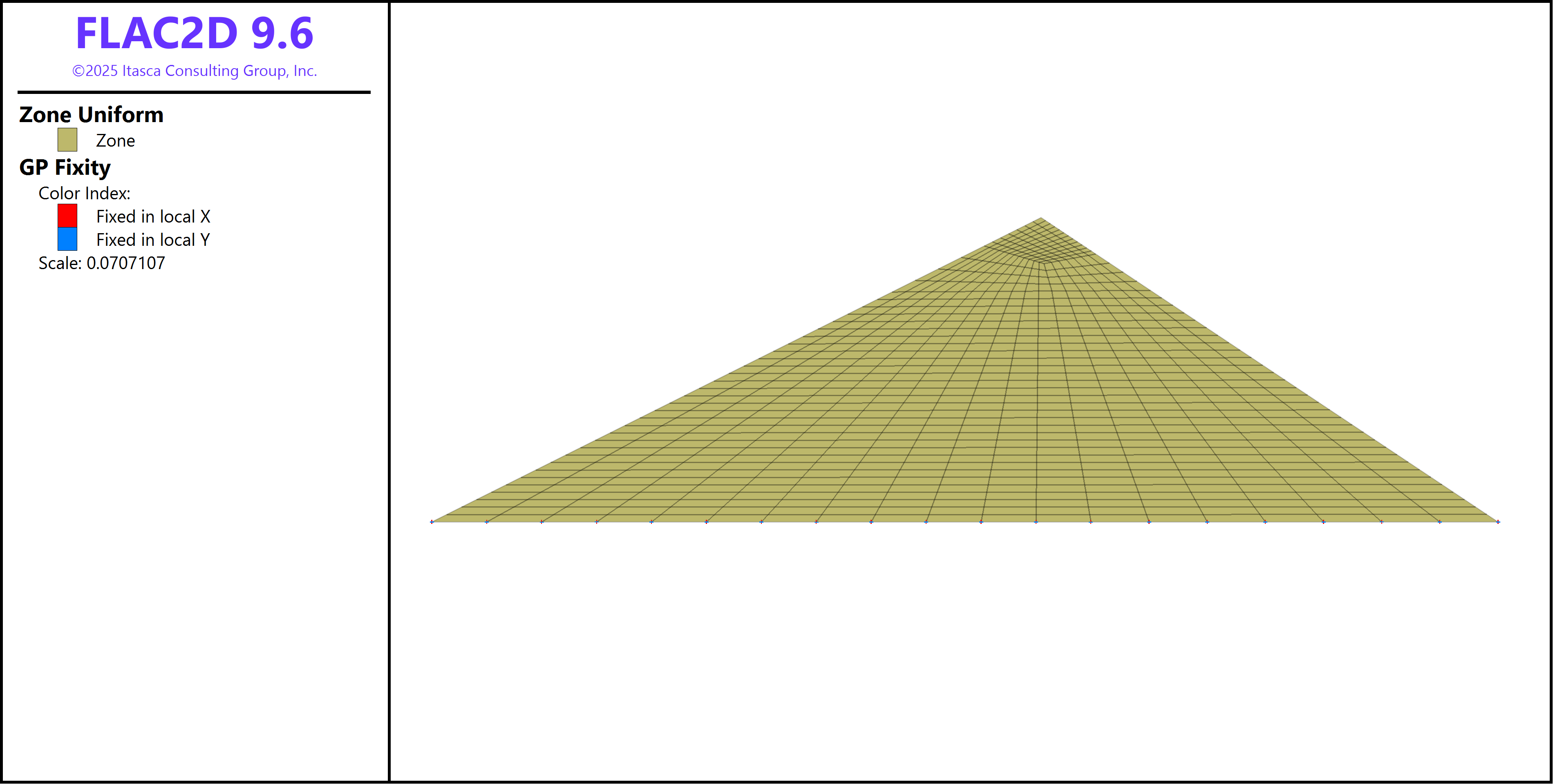
Figure 1: Model geometry and boundary conditions at the base.
Gravity and initial stresses are not considered in this analysis. The first step of this example involves applying a horizontal load of 1000 kN/m to the dam crest (using FISH to identify the gridpoint coinciding with the crest), followed by solving to static equilibrium. The point load is added as an additional nodal force:
[global gp = gp.near((90.0,45.0))]
[gp.force.load(gp)->x = 1.0e6]
The second step is the free vibration analysis where the point load is removed and the dam is allowed to vibrate freely in the absence of damping. Displacements in this step account for the displacements obtained in the static step. During the analysis, the total dynamic time and horizontal displacement at the crest are monitored (Figure 2). As a post-processing step, the first and second natural frequencies of the dam structure are found by transforming the recorded horizontal displacement from the time domain into the frequency domain.
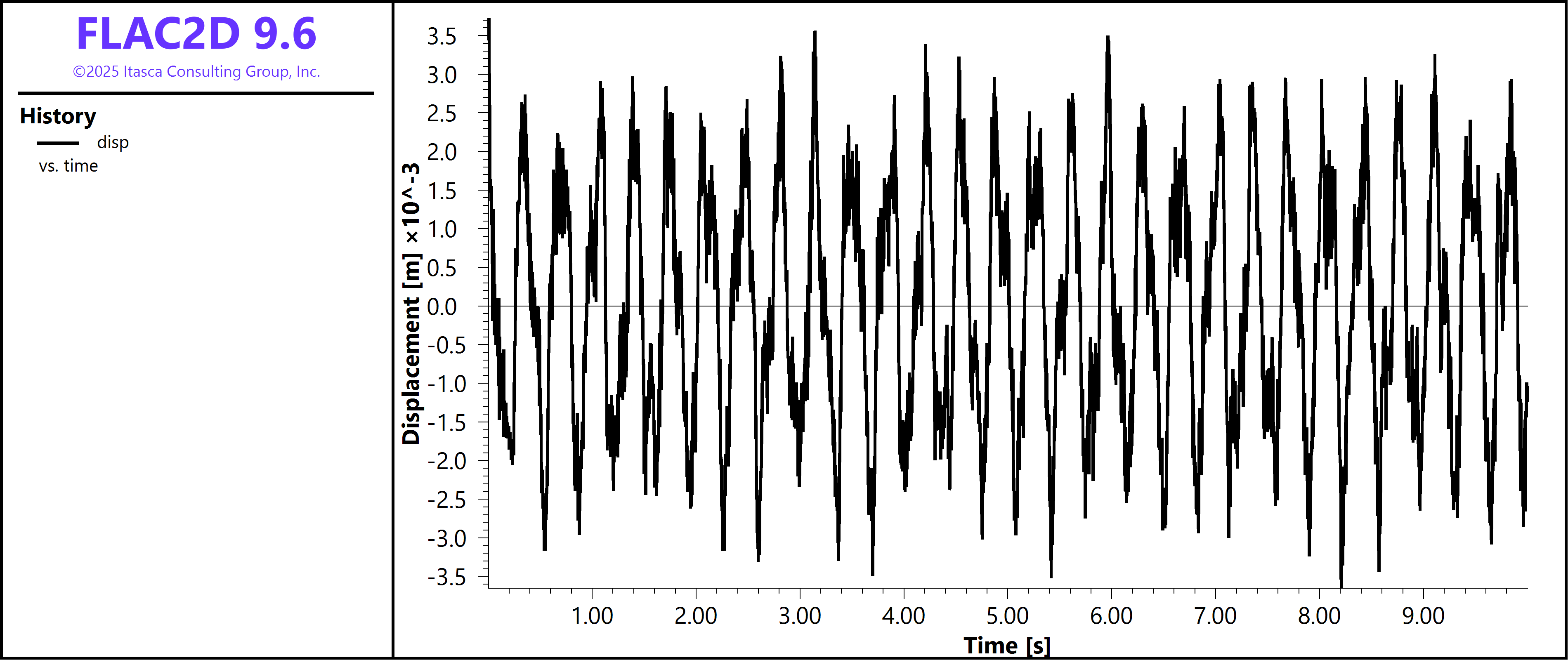
Figure 2: Horizontal displacement history at the dam crest.
The natural frequency of vibration of the dam structure can be estimated, analytically, using the following equation:
where \(\bar{V_s}\) is the average shear wave velocity of the soil in the dam, \(H\) is the height of the dam, \(\beta_n\) is the nth root of a period relation (given by tabulation tables in Kramer (1996)), and \(m\) is a material constant that describes shear modulus increase with depth according to \(G=G_{b}\left(z/H\right)^m\) where \(G_{b}\) is the shear modulus at the base and \(z\) is the depth from the crest. In this example, the elastic moduli are homogeneous and, therefore, \(m\) is taken equal to zero. The first two roots of the period relation are \(\beta_1=2.404\) and \(\beta_2=5.520\). Using these values, the first two natural frequencies of the dam structure are estimated as 3.11 Hz and 7.14 Hz, respectively. The power spectrum vs. frequency obtained from FLAC2D is shown in Figure 3. The conversion from the time to frequency domain involves a Fast Fourier Transform (FFT) of the recorded horizontal displacement at the dam crest. The first two natural frequencies correspond to the distinct peaks in the power spectrum. The results from FLAC2D are in close agreement with the analytical values which are plotted as points below.
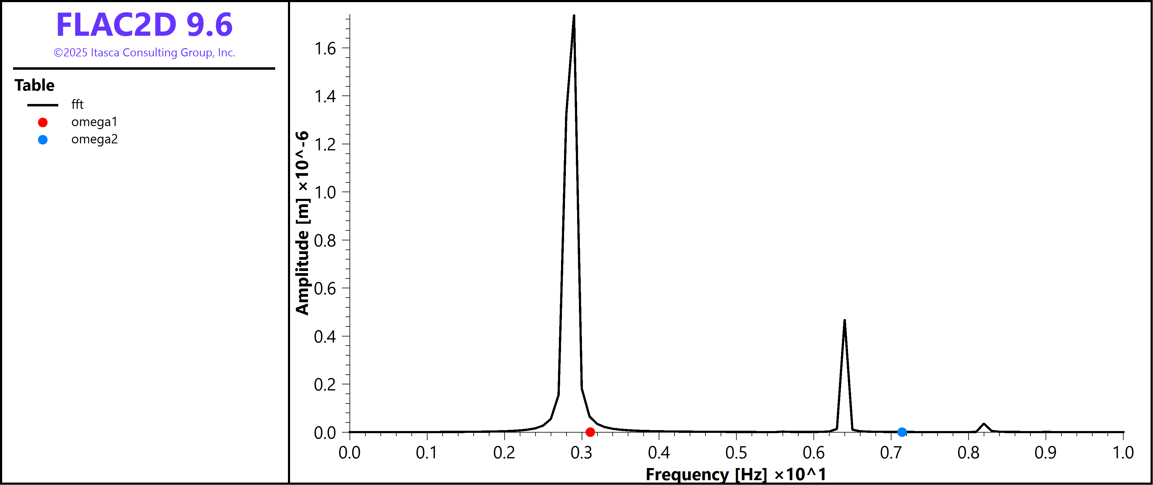
Figure 3: Power spectrum of dam vibrations in the frequency domain obtained from FLAC2D and compared to analytical solutions of the first two natural frequencies.
References
Kramer, S. L. Geotechnical Earthquake Engineering. Prentice Hall, New Jersey (1996).
Data File
vibration.dat
model new
model large-strain off
model configure dynamic
model dynamic active off
;
program call "geom.dat"

; -------------------------------------- ;
; Apply force
; -------------------------------------- ;
[global rho = 1834.86]
[global bulk = 327.3e6]
[global shear = 245.5e6]
zone cmodel assign elastic
zone property density [rho] bulk [bulk] shear [shear]

zone gridpoint fix velocity-y 0
zone gridpoint fix velocity-x 0 range group 'Skin=Bottom'

[global gp = gp.near((90.0,45.0))]
[gp.force.load(gp)->x = 1.0e6]

model solve ratio-local 1e-5

; -------------------------------------- ;
; Release force
; -------------------------------------- ;
[gp.force.load(gp)->x = 0.0]

model dynamic active on
history interval 10
model history name 'time' dynamic time-total
zone history  name 'disp' displacement-x ...
    gridpointid [gp.id(gp)]

model solve time-total 10
history export 'disp' vs 'time' table 'disp'

; -------------------------------------- ;
; Numerical natural frequencies
; -------------------------------------- ;
fish define FFT(tab)
    global freq = table.fft(tab)
    loop i (1, list.size(freq))
        table.value('fft',i) = freq(i)
    endloop
end
[FFT('disp')]

; -------------------------------------- ;
; Empirical natural frequencies
; -------------------------------------- ;
fish define ENF
    local Vs    = math.sqrt(shear/rho)
    local H = 45.0
    local m = 0
    global omega1 = (Vs*2.404)*(4+m)*(2-m) / (16*H*math.pi)
    global omega2 = (Vs*5.520)*(4+m)*(2-m) / (16*H*math.pi)
    table.value('omega1',1) = (omega1,0)
    table.value('omega2',1) = (omega2,0)
end
[ENF]

model save 'vibration.sav'
Endnote
| Was this helpful? ... | Itasca Software © 2026, Itasca | Updated: Feb 07, 2026 |
