Unsaturated Flow around a Drift (FLAC2D)

Problem Statement

Example Application

This project reproduces a two-phase flow example from FLAC 8.1. The project file for this example may be viewed/run in FLAC2D.[1] The main data file used is shown at the end of this example.

How To Read and Use Examples

Under unsaturated conditions, underground excavation can serve as an obstacle to the flow. This example analyzes unsaturated seepage flow around a system of horizontal drifts located 60 m apart, and situated 30 m below ground level. The diameter of the drifts is 5 m. Surface water is infiltrating at a steady rate, \(q_0\), of 2 × 10^-8 m/s. The phreatic surface level is at a depth of 60 m. The purpose of the simulation is to determine the saturation distribution around the drifts when steady-state conditions are reached.

Modeling Procedure

Model Geometry and Boundary Conditions

By symmetry, half of a drift is considered for this problem. The model is created using primitives; specifically zone create2d sector-quad followed by zone reflect. This results in a radial grid of 1250 zones (Figure 1). A discharge boundary condition is applied at the top of the model (ground level), a constant pressure is assigned at the bottom of the grid (phreatic surface), and a seepage condition is declared at the drift boundary. There is no seepage boundary condition in FLAC2D, as in FLAC 8.1, so this is implemented with a small FISH function that checks the nodes on the tunnel surface each timestep. If the pressure becomes positive, then the boundary changes from impermeable to permeable (fixed pore pressure).

The lateral boundaries are impermeable to water flow (symmetry conditions). The initial saturation corresponds to one-dimensional gravity flow with constant specific discharge, \(q_0\) (saturation = 0.42).

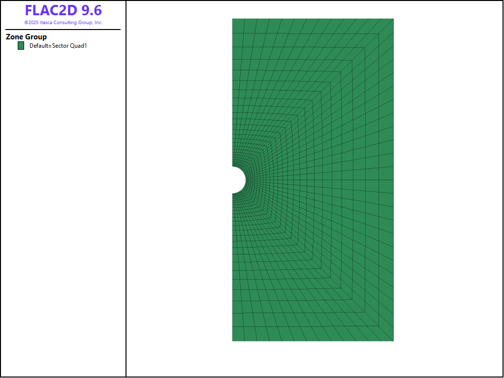
Figure 1: Model geometry

Properties

The material is assumed to be a low porosity rock. The fluid properties assumed for this problem are listed in Table 1. Note that the fluid modulus is lower than the actual modulus of fluid since the problem is only solved to steady state. Note also that zone fluid steady-state command is not used because of the changing boundary conditions required to simulate the seepage boundary.

Table 1: Fluid Properties

Property	Value
Fluid Density (kg/m³)	1000
Fluid modulus (MPa)	0.01
Porosity	5 × 10⁻⁵
Hydraulic conductivity (m/s)	10⁻⁵
van Genuchten parameter m	0.63
van Genuchten parameter n	2.70
van Genuchten parameter \(P_0\) (MPa)	0.001

The van Genuchten parameters are taken from the original FLAC 8.1 example that uses two-phase flow. For this example, an equation relating negative pore pressure (\(P_w\)) to saturation (\(S_e\)) is given:

\[-P_w = P_0 \left[S_e^{-1/a} - 1 \right]^{1-a}\]

where \(P_0\) is a reference pressure and \(a\) is a fitting parameter. This can be rearranged to give the equation for saturation versus pressure as shown here and reproduced below:

\[\hat{s} = \frac{1}{\left[ 1 + \left( \frac{\psi}{\psi_r} \right)^n \right]^m}\]

In this equation, \(m\) is equivalent to \(a\), \(n\) is equivalent to \(1 \over {1-a}\), \(\psi\) and \(\psi_r\) are equivalent to \(P_w\) and \(P_0\). The curve for these parameters is shown in Figure 2.

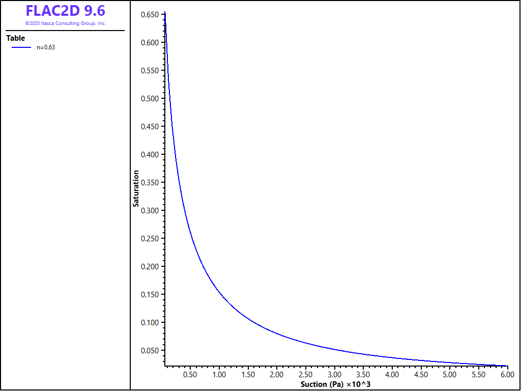
Figure 2: van Genuchten soil-suction curve for m = 0.63, n = 2.7 and \(P_0\) = 1 kPa.

In addition, the FLAC 8.1 example uses the following relationship between relative permeability (\(\kappa^w\)) and saturation (\(S_w\)):

\[\kappa^w = S_w^b \left[1-\left(1-S_w^{1/a} \right)^a \right]^2\]

In the example, \(b\) = 0.5. This permeability relationship is implemented in FLAC2D by creating a table of values that is input to the zone fluid permeability-saturation command. The resulting table is shown in Figure 3.

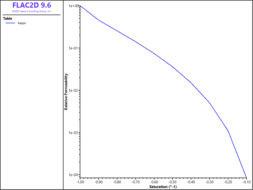
Figure 3: Relationship between relative permeability and saturation.

Results

Figure 4 shows the steady-state contours of saturation for the simulation. Pore pressure contours and flow vectors are given in Figure 5. As may be seen in the plots, water is deflected from the drift roof, and “drip lobes” in which saturation and flow velocity are increased (compared to the initial steady situation) are formed. A dry shadow is formed, sheltered by the cavity. These features are described in the context of Richard’s equation (see Philip et al. 1989) and a relative permeability exponential law.

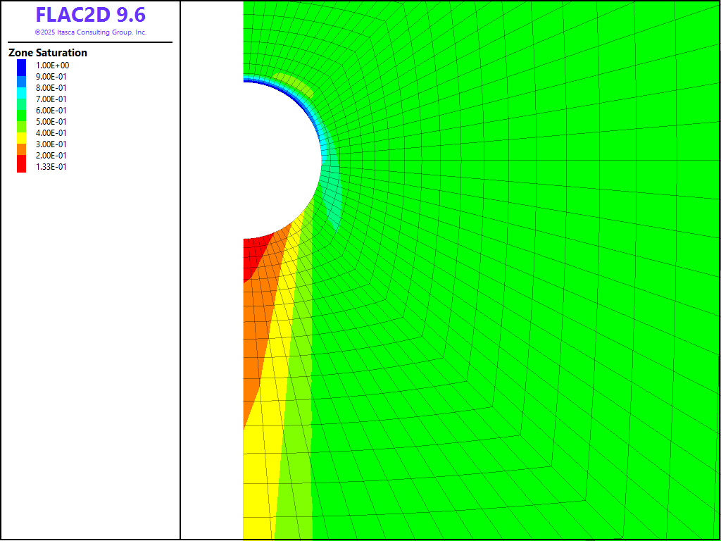
Figure 4: Contours of saturation

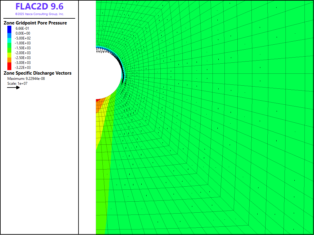
Figure 5: Pore pressure contours and flow vectors

References

Philip, J. R., J. H. Knight and R. T. Waechter. “Unsaturated Seepage and Subterranean Holes: Conspectus, and Exclusion Problem for Circular Cylindrical Cavities”, Water Resources Research, 25(1), 16-28 (1989).

Data Files

drift.dat

model new
model configure fluid-flow

; create geometry
zone create2d sector-quad point 0 (0,0) point 1 (30,0) point 2 (0,30) ...
  point 3 (30,30) point 4 (2.5,0) point 5 (0,2.5) size 10 25 25 ratio 1 1 1.1
  
zone reflect normal 0,1

; fluid properties
model gravity 9.81
zone fluid-density 1000
zone fluid property porosity 5e-4 hydraulic-conductivity 1e-6
zone fluid property fluid-modulus 1e4
[a = 0.630]  ; a parameter from FLAC 8.1
zone fluid unsaturated van-genuchten [1/(1-a)] [a] 1000

; make a table for relative permeability
[b = 0.5]
fish define kappa
  local tab = table.create('kappa')
  loop local i (1,10)
    local sat = i*0.1
    table(tab,sat) = (sat^b)*(1-(1-sat^(1/a))^a)^2
  end_loop
end
[kappa]

zone fluid permeability-saturation table 'kappa'

; initial conditions
zone gridpoint initialize saturation 0.42

; boundary conditions
zone face skin
zone face apply discharge 2e-8 range group 'Top'
zone face apply pore-pressure 0 range group 'Bottom'
zone gridpoint initialize saturation 1 range group 'Bottom'   ; ??

; fish function to implement seepage boundary condition
; when saturation goes to 1, flow is possible through the boundary
fish define get_gps
  drift_gps = list
  loop foreach local gp gp.list
    if gp.isgroup(gp,'West3','Skin')
      drift_gps('end') = gp
    endif
  end_loop
end
[get_gps]

fish operator set_seepage(gp)
  ;if gp.sat(gp) >= 1.0
  if gp.pp(gp) >= 0
    gp.pp.fix(gp) = true
  end_if
end

; call every step
fish callback add [set_seepage(::drift_gps)] -1 

;zone fluid implicit on servo active on
model solve-fluid time 3e5
model save 'drift'

Endnote

[1]

This example is listed under the present document title in the i Examples dialog (use the menu command Help -> Examples… to access).