Munson-Dawson (MD)Model
Munson and Dawson (1979, 1982) and Munson et al (1989) developed the “Munson-Dawson” (MD) model (also known as the “Multimechanism Deformation” model) for the creep behavior for rock salts in nuclear storage caverns, subsurface mines, and waste repositories. Both steady-state and transient strain rates are treated in the MD model. The steady-state strain rate of the MD model consists of three components: dislocation climb, an undefined mechanism, and dislocation glide. The transient strain rate captures recovery effect where the rate of strain hardening is stress dependent. The original MD model featured some drawbacks, including less accurate creep behavior at low equivalent stresses less than 8 MPa, lack of the flexibility to capture true triaxial creep measurements, and frequently unstable numerical performance of implementation. The present implementation is based on the enhanced version (Reedlunn, 2018) with the following features.
A more flexible Hosford stress measure has been adopted, enabling the accommodation of both Tresca and von-Mises stress states as specific instances, contingent upon the assignment of a material parameter.
New transient and steady-state rate terms are added to capture salt’s creep behavior at low equivalent stresses (below about 8 MPa).
The steady-state strain rate consists of three components.
Model Description
The MD model assumes that plastic deformation of intact salt is isochoric and only occurs in the presence of shear stress, \(\sigma_e\), and the volumetric part is purely elastic.
The viscoplastic strain rates are defined as
where \(\dot{\varepsilon}^{vp}_{ij}\) is the viscoplastic strain-rate tensor, \(\sigma_e\) is a measure of effective stress, \(\sigma_{ij}\) is the effective stress tensor, \(\dot{\varepsilon}_s\) is the steady-state equivalent viscoplastic strain rate, and \(F\) is a scalar factor that will be explained later.
The original MD model adopted von-Mises stress \(\sigma_{VM}\) for \(\sigma_e\). Later Tresca stress was used. This version adopts the more flexible Hosford (1972) stress defined by
where \(\sigma_i\) (i = 1,2,3) are the principal effective stresses and \(a\) is a material parameter. For \(a=1\) it degenerates into the Tresca stress and for \(a=2\) it is equivalent to the von-Mises stress, and a range of behaviors in-between for \(1 \le a \le 2\). Alternatively, the Tresca stress can be reproduced with \(a=\infty\), the von-Mises stress with \(a=4\), and the behavior range can be in-between with \(4 \le a \le \infty\) (see Figure 1). Restricting \(a \ge 4\) is recommended (Reedlunn, 2018) to avoid possible numerical singularity, particularly during the calculation of derivative of Hosford stress to the principal stress. In this model, the parameter \(a\) is an input material property that must be calibrated. It has been shown that this parameter is quite sensitive to the simulated results of an example underground cavern drift undergoing creep deformation (Cheng, 2024).
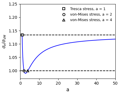
Figure 1: Schematics of the ratio of Hosford stress to von-Mises stress, assuming \(\sigma_1 = -4\), \(\sigma_2 = -2\) and \(\sigma_3 = -1\) as an example.
The steady-state equivalent viscoplastic strain rate is the sum of four mechanisms:
and the first three ones \(\dot{\varepsilon}_i\) (i = 0,1,2) are defined as
and the last one is defined as
where \(A_i\), \(B_i\), \(Q_i\), \(n_i\), \(\sigma_0\) and \(q\) are all model parameters. \(Q_i\) are the activation energies, \(R\) (= 8.314 J/[K mol]) is the universal gas constant, \(T\) is the absolute temperature, \(G\) is the shear modulus. \(H()\) is the Heaviside step function. The new mechanism (i = 0) is added upon the original mechanisms 1 to 2 to enhance the behavior at low equivalent effective stress less than 8 MPa.
As explained in Reedlunn (2018), an actual micro-mechanical mechanism responsible for the creep behavior at low equivalent stresses has not yet been identified. Therefore, the newly introduced Mechanism 0 is assigned the same mathematical form as Mechanisms 1 and 2. Mechanism 1 is intended to represent dislocation climb, which dominates at high temperatures and low equivalent stresses. Mechanism 2 governs behavior at low temperatures and medium equivalent stresses. Although the micro-mechanical origin of Mechanism 2 remains unclear, recent work by Hansen (2014) suggests that cross-slip may be responsible. Regardless, the macroscopic behavior associated with this mechanism has been well characterized. Mechanism 3 models dislocation glide, which becomes active only when the equivalent stress \(\sigma_e\) exceeds \(\sigma_0\), as indicated by the Heaviside function \(H(\sigma_e - \sigma_0)\). The parameters \(B_i\) are typically chosen to ensure a smooth transition to Mechanism 3 at \(\sigma_0\).
The change rate of transient equivalent viscoplastic strain component \(\dot{\varepsilon}_t\) (so \(\dot{\varepsilon}_t + \dot{\varepsilon}_s = \dot{\varepsilon}_{vp}\)) is with the evolutionary equation:
where \(\varepsilon_t^*\) is the transient strain limit, \(\Delta\) and \(\delta\) are the work-hardening and recovery parameters, respectively. The exponent \(\chi\) is treated as an input parameter that can be customized by the user, with a default value of 2. Cheng (2024) shows that the sensitivity of \(\chi\) is pronounced only during the transient stage, while it becomes negligible when approaching the steady-state phase.
The transient strain limit is defined by
where \(K_i\), \(c_i\), and \(m_i\) are material constants. Again, this enhanced version added a second mechanism i = 0 to capture the transient creep at low equivalent stress.
The work-hardening (\(\Delta\)) and recovery (\(\delta\)) parameters are described through functions:
where \(\alpha_h\), \(\beta_h\), \(\alpha_r\) and \(\beta_h\) are material parameters.
Implementation
The incremental for of Eq. (1) is given by
An explicit algorithm is used which implies that any variable at time \(t\) is known and in this constitutive level the time increment \(\Delta t\) and strain increment \(\Delta \varepsilon_{ij}\) are known as well. We need to solve the updated stress at time \(t + \Delta t\).
The updated deviatoric stress is
where \(\sigma_e\) is unknown and \(\dot{\varepsilon}_s\) is a function of \(\sigma_e\). Here an iteration method is used:
(1). Initialize an intermediate stress \(S^m_{ij} = S^t_{ij}\) and the iteration index \(I_{iter}\) = 1.
(2). Calculate the Hosford stress and its derivative in terms of \(S^m_{ij}\).
(3). Calculate \(\dot{\varepsilon}_s\).
(4). Update \(S^{t + \Delta t}_{ij}\) based on Eq. (12).
(5). Update \(S^m_{ij} = (S^t_{ij} + S^{t + \Delta t}_{ij})/2\), and \(I_{iter}\) = \(I_{iter}\) + 1.
(6). Go back to (2) until a convergence criterion or \(I_{iter}\) reaches an allowable maximum iteration number \(I^{max}_{iter}\).
(7). Return \(S^{t + \Delta t}_{ij}\), end the current time step, and pass updated variables to the next time step.
The total number of iterations, \(I^{max}_{iter}\), can range from a minimum of 1 to more than 10. A higher \(I^{max}_{iter}\) value is expected to yield more accuracy, but this comes at the cost of increased computational time. However, as evidenced by Cheng (2024), \(I^{max}_{iter}\) = 1 is generally numerically sufficient. This sufficiency is due to the small allowable timestep, prescribed by the global explicit algorithm used in FLAC, which is constrained by the maximum permissible timestep. Based on the outcomes of the testing, \(I^{max}_{iter}\) = 1 is used in the implementation, as it requires the fewest calculation steps and is the most efficient numerically. Alternately, more accuracy can be achieved by reducing time step.
The volumetric behavior is elastic since this model considers only the creep effect from deviatoric stress. The updated isotropic part of stress is given by
(13)\[ \sigma^{t + \Delta t}_v = \sigma^{t}_v + 3K \Delta \varepsilon_v\]
where \(K\) is the bulk modulus, \(\sigma_v\) and \(\varepsilon_v\) are volumetric stress and strain, respectively.
In the described algorithm, the Hosford stress, which is formulated in terms of the principal stresses, necessitates the conversion of stress/strain tensors into the principal stress/strain space. This transformation simplifies the calculation process by directly utilizing the principal stress components.
This enhanced MD model has been implemented based on a numerical framework (FLAC2D, FLAC3D and 3DEC) that utilizes an explicit algorithm characterized by small time steps. This approach is governed by the principle that the calculation front advances faster than the traveling wave. One of the main advantages of this explicit algorithm is that it eliminates the need for global stiffness and obviates the necessity for second derivatives of the yield or potential function, which are crucial in an implicit algorithm.
One Creep Timestep
While the user has the flexibility to set the timestep, this setting is not arbitrary. For a system to consistently maintain quasi-static mechanical equilibrium (e.g., in FLAC3D) as required in a creep simulation, the time-dependent stress changes by the constitutive law must be small relative to the strain-dependent stress changes. If this is not the case, out-of-balance forces will become significant, and inertial effects may compromise the accuracy of the solution. In this enhanced MD model, the creep processes are governed by the deviatoric stress state. An estimate for the maximum creep timestep for numerical accuracy can be expressed as the ratio of the material viscosity to the shear modulus. The ratio of material viscosity is approximated as the ratio of the equivalent Hosford stress to the creep strain rate. The allowable maximum creep time step can thus be estimated (Cheng 2024) as
(14)\[ \Delta t^{max}_{cr} = \dfrac{\sigma_e}{F \dot{\varepsilon}_s}\]
At the start of creep simulation \(\dot{\varepsilon}_s\) may be large and thus \(\Delta t^{max}_{cr}\) should be small; approaching steady state \(\dot{\varepsilon}_s\) is close to zero and thus \(\Delta t^{max}_{cr}\) can be very large.
In practice, the timestep can be set to a constant value by the user or adjusted automatically by the software. When set to adjust automatically, the timestep can decrease if the maximum unbalanced force exceeds a certain threshold and increases when it falls below another level. This threshold is typically defined as the ratio of the maximum unbalanced force to the average gridpoint force. To determine typical out-of-balance force criteria for the problem at hand, one can observe the out-of-balance force near equilibrium in the initial phase of the problem when only elastic effects are present. Often, optimal performance is achieved by gradually increasing or decreasing the timestep. Generally, the timestep starts at a low value to manage transients, such as excavation, and then is increased as the simulation progresses. If a new transient occurs, it may be necessary to manually decrease the timestep, allowing it to later increase automatically again. In any case, the maximum timestep should not exceed the value estimated in Eq. (14); otherwise, an error message will be triggered.
Property List
Category |
Names |
Default |
|---|---|---|
Elasticity |
bulk (\(K\)) |
|
shear (\(G\)) |
||
Stress Measure |
hosford (\(a\)) |
4.0 |
Temperature |
temperature (\(T\)) |
|
Creep |
A-i (\(A_i\), i = 0,1,2) |
0.0 |
B-i (\(B_i\), i = 0,1,2) |
0.0 |
|
activation-ratio-i (\(Q_i/R\), i = 0,1,2) |
0.0 |
|
n-i (\(n_i\), i = 0,1,2) |
0.0 |
|
stress-constant (\(q\)) |
||
stress-limit (\(\sigma_0\)) |
||
K-i (\(K_i\), i = 0,1) |
0.0 |
|
c-i (\(c_i\), i = 0,1) |
0.0 |
|
m-i (\(m_i\), i = 0,1) |
0.0 |
|
alpha-hardening (\(\alpha_h\)) |
0.0 |
|
beta-hardening (\(\beta_h\)) |
0.0 |
|
alpha-recovery (\(\alpha_r\)) |
0.0 |
|
beta-recovery (\(\beta_r\)) |
0.0 |
|
f-exponent (\(\chi\)) |
2.0 |
|
Read-Only |
steady-rate (\(\dot{\varepsilon}_s\)) |
|
transient-rate (\(\dot{\varepsilon}_t\)) |
||
internal-variable (\(\varepsilon_t^*\)) |
||
creep-strain-rate-ij (\(\dot{\varepsilon}^{vp}_{ij}\), i,j=1,2,3) |
Acknowledgment
The implementation of this model was partially sponsored by RESPEC.
References
Cheng, Z. Implementation and Verification of Enhanced Munson-Dawson Creep Model for Rock Salt. In US Rock Mechanics/Geomechanics Symposium (D041S047R003), ARMA (2024).
Hansen, F. D. Micromechanics of Isochoric Salt Deformation. In: 48th US Rock Mechanics/Geomechanics Symposium. ARMA. (2014).
Hosford, W.F. A generalized isotropic yield criterion. Journal of Applied Mechanics, 39(2), 607-609 (1972).
Munson, D.E., & Dawson, P. Constitutive model for the low temperature creep of salt (with application to WIPP) (Tech. Rep. SAND79-1853). Sandia National Laboratories, Albuquerque, NM, USA (1979).
Munson, D.E., & Dawson, P. Transient creep model for salt during stress loading and unloading (Tech. Rep. SAND82-0962). Sandia National Laboratories, Albuquerque, NM, USA (1982).
Munson, D.E., Fossum, A.F., & Senseny, P.E. Advances in resolution of discrepancies between predicted and measured in situ WIPP room closures (Tech. Rep. SAND88-2948). Sandia National Laboratories, Albuquerque, NM, USA (1989).
Reedlunn, B. Enhancements to the Munson-Dawson model for rock salt (No. SAND-2018-12601). Sandia National Laboratories, Albuquerque, NM, USA (2018).
Examples
Munson-Dawson Model: Triaxial Test
Munson-Dawson Model: Pure Shear Test
Munson-Dawson Model: Biaxial Test
Munson-Dawson Model: Underground Drift
munson-dawson Model Properties
Use the following keywords with the zone property command to set these properties of the Munson-Dawson model.
- a-0 f
parameter \(A_0\)
- a-1 f
parameter \(A_1\)
- a-2 f
parameter \(A_2\)
- activation-ratio-0 f
parameter \(Q_0/R\)
- activation-ratio-1 f
parameter \(Q_1/R\)
- activation-ratio-2 f
parameter \(Q_2/R\)
- alpha-hardening f
parameter \(\alpha_h\)
- alpha-recovery f
parameter \(\alpha_r\)
- b-0 f
parameter \(B_0\)
- b-1 f
parameter \(B_1\)
- b-2 f
parameter \(B_2\)
- beta-hardening f
parameter \(\beta_h\)
- beta-recovery f
parameter \(\beta_r\)
- bulk f
elastic bulk modulus, \(K\)
- c-0 f
parameter \(C_0\)
- c-1 f
parameter \(C_1\)
- k-0 f
parameter \(K_0\)
- k-1 f
parameter \(K_1\)
- m-0 f
parameter \(m_0\)
- m-1 f
parameter \(m_1\)
- n-0 f
parameter \(n_0\)
- n-1 f
parameter \(n_1\)
- n-2 f
parameter \(n_2\)
- shear f
elastic shear modulus, \(G\)
- stress-limit f
stress limit, \(\sigma_0\)
- stress-constant f
stress constant, \(q\)
- temperature f
temperature, \(T\).
- f-exponent f (a)
parameter, \(\chi\), with a default value 2.0.
- hosford f (a)
Hosford parameter, \(a\), with a default value 4.0. Allowable value is no less than 2.0. If \(a = 2.0\) or \(a = 4.0\), the Hosford stress degrades to the von-Mises stress. If \(a = \infty\) (practical, a large value, e.g., \(a = 100\) is sufficient) the Hosford stress degrades to the Tresca stress.
- internal-variable f (r)
current transient strain limit, \(\varepsilon_t^*\).
- steady-rate f (r)
current steady creep strain rate, \(\dot{\varepsilon}_s\).
- transient-rate f (r)
current transient creep strain rate, \(\dot{\varepsilon}_t\).
- creep-strain-rate-11 f (r)
current creep strain rate, \(\dot{\varepsilon}^{vp}_{11}\).
- creep-strain-rate-22 f (r)
current creep strain rate, \(\dot{\varepsilon}^{vp}_{22}\).
- creep-strain-rate-33 f (r)
current creep strain rate, \(\dot{\varepsilon}^{vp}_{33}\).
- creep-strain-rate-12 f (r)
current creep strain rate, \(\dot{\varepsilon}^{vp}_{12}\).
- creep-strain-rate-13 f (r)
current creep strain rate, \(\dot{\varepsilon}^{vp}_{13}\).
- creep-strain-rate-23 f (r)
current creep strain rate, \(\dot{\varepsilon}^{vp}_{23}\).
Key
- (a) Advanced property.
This property has a default value; simpler applications of the model do not need to provide a value for it.
- (r) Read-only property.
This property cannot be set by the user. Instead, it can be listed, plotted, or accessed through FISH.
| Was this helpful? ... | Itasca Software © 2026, Itasca | Updated: Feb 07, 2026 |
