Embankment Consolidation (Mohr-Coulomb) (FLAC2D)
Problem Statement
Note
To view this project in FLAC2D, use the menu command . Choose “Embankment Consolidation (Mohr-Coulomb)” and select “EmbankmentConsolidation.prj” to load. The project’s main data files are shown at the end of this example.
This example illustrates the use of FLAC2D to analyze soil consolidation underneath an embankment by utilizing a loosely coupled fluid-mechanical approach. This problem is common in geotechnical engineering and arises when road embankments are to be constructued over saturated soils in a short amount of time. Due to excess pore pressure generation of low permeability soils, the embankment is usually constructed in multiple lifts. The embankment is constructed in four lifts over 60 days, during which, pore pressure dissipation and soil consolidation takes place. A load representing traffic is placed on the top of the embankment following the last lift. The full construction sequence is given in Table 1. The numerical model initially contains the four embankment layers but are nulled prior to gravity initialization. The null zones are considered not present for most purposes during calcuations or plotting. Each embankment layer is un-nulled at the time of construction, providing an additional load due to the weight associated with the layer.
Sequence Step |
Description |
Duration (days) |
Solution Type |
|---|---|---|---|
01 |
Initilization |
0 |
Mechanical |
02 |
Construct lift 1 |
1 |
Fluid-Mechanical |
03 |
Construct lift 2 |
9 |
Fluid-Mechanical |
04 |
Construct lift 3 |
10 |
Fluid-Mechanical |
05 |
Construct lift 4 |
40 |
Fluid-Mechanical |
06 |
Apply traffic load |
5 |
Fluid-Mechanical |
The model is constructed in Sketch and groups are assigned to the different layers after the geometry is defined. Three soil layers are present in the model (from surface to depth): a high permeability silty sand, a low permeability silty sand, and a dense silty sand. The model geometry and soil layers are shown in Figure 1.
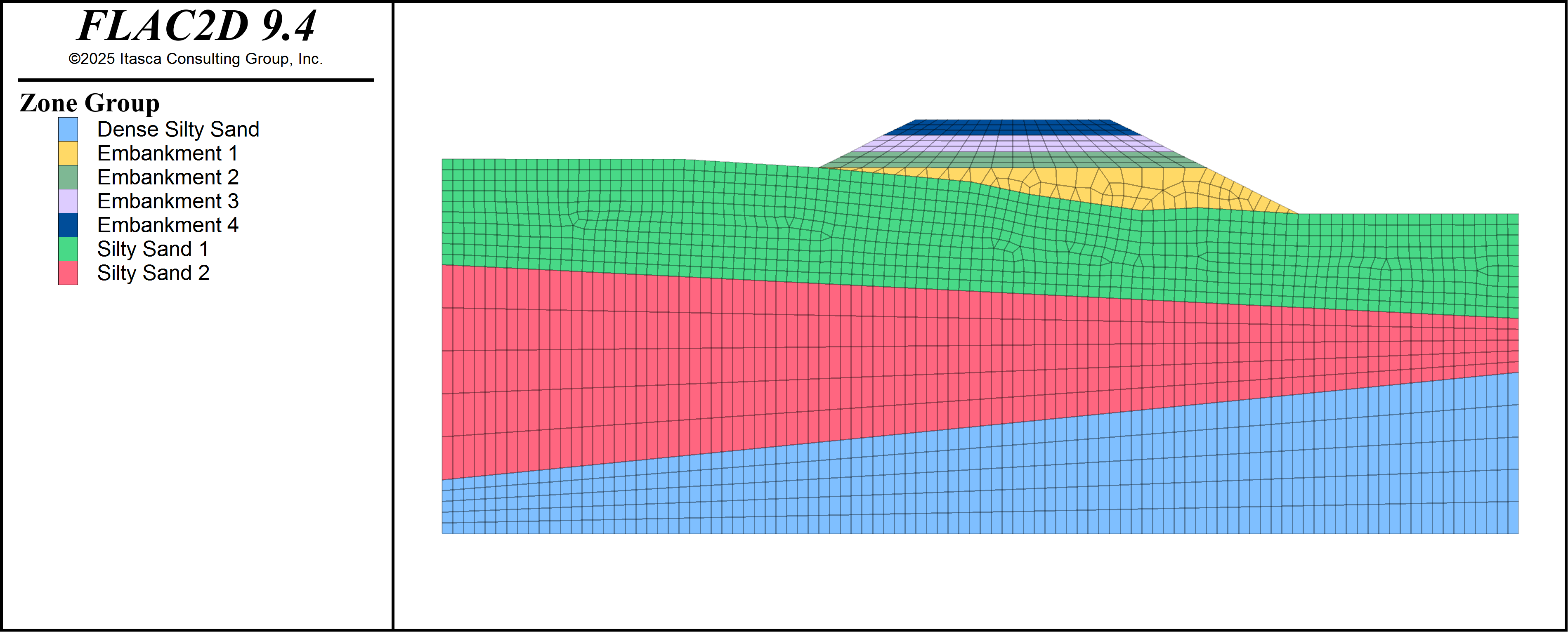
Figure 1: Model geometry, soil layers, and embankment lifts.
The soil layers are modeled with a Mohr-Coulomb constitutive law while the embankment is elastic. Furthermore, the embankment is considered impermeable, i.e., excess pore pressure due to embankment loading must dissipate in the sand layers. Material properties are given in Table 2. Because the confined stiffness is constant in the elastic region and this model is mostly elastic, the loosely coupled modeling approach closely approximates the fully coupled system. The loosely coupled approach performs an undrained step with the “true” fluid modulus (using zone fluid modulus-automatic and zone fluid property pore-pressure-generation on) followed by a drained step using the commands zone fluid modulus-scale and model solve-fluid-decoupled.
Property |
Embankment |
Silty Sand 1 |
Silty Sand 2 |
Dense Silty Sand |
|---|---|---|---|---|
Dry density (kg/m3) |
1335 |
1835 |
1835 |
1835 |
Porosity (-) |
0.5 |
0.5 |
0.5 |
0.5 |
Bulk modulus (kPa) |
11.11 |
20.83 |
11.11 |
13.89 |
Shear modulus (kPa) |
8.33 |
9.62 |
8.33 |
10.42 |
Friction angle (deg) |
32 |
33 |
35 |
|
Cohesion (kPa) |
0.25 |
0.1 |
0.1 |
|
K0 (-) |
0.8 |
0.5 |
0.5 |
0.5 |
Conductivity (m/s) |
Impermeable |
\(5\times 10^{-6}\) |
\(2\times 10^{-8}\) |
\(1\times 10^{-7}\) |
Staged Construction Sequence
As previously mentioned, the embankment is constructed in four lifts over a period of 60 days. Each lift includes the following steps:
The lift is un-nulled with
zone nullset tofalseand the full density is assigned.Stress is initialized in the embankment lift with K0 conditions with
zone initialize-stresses.The “true” fluid stiffness is set using
zone fluid modulus-automatic. (This assumes the fluid is essentially incompressible relative to the soil and therefore sets the fluid modulus to be 20x stiffer than the soil stiffness).Pore pressure generation is activated in the soil layers with
zone fluid pore-pressure-generation.The model is solved to undrained static equilibrium with
model solve-static. This step involes zero time, i.e., it is considered the instantaneous response.The newly un-nulled embankment layer is made impermeable with
zone fluid cmodel assign inactive.The fluid stiffness is scaled to account for skeleton compressibility with
zone fluid modulus-scale.The model is solved for a period of time to allow for pore pressure dissipation and consolidation with
model solve-fluid-decoupled. The time in this step is physical and represents the construction time. This example uses 1 day for the first lift, 9 days for the second lift, 10 days for the third lift, and 40 days for the fourth lift.
This process is repeated for each lift until all lifts have been constructed. The main idea of the steps is to honor the staged construction sequence that incorporates a physical time element. Note that for large embankments or for non-linear materials, this process may need to be further refined into sub-steps. The sub-steps would then ramp the density of each lift from a small multiplier to the full value. Finally, if the consolidation coefficient is known for the soil layers, then the preferred method to set the fluid stiffness during consolidation is with zone fluid property consolidation-coefficient.
Boundary and Initial Conditions
The first step is to initialize the model with gravity, K0 conditions, and a hydrostatic pore pressure. The water table is initially a few meters below the ground surface (\(y = -12\) m). Saturation is assumed to be 1 everywhere in the model. This is something done to simplify the model and place emphasis on the consolidation process without incorporating unsaturated fluid flow models. Regions above the water table are allowed to have negative pore pressures, but have no impact on effective stress calculations as this example uses an effective stress cutoff of 0.
The mechanical boundary conditions are: roller constraints on the lateral boundaries and a fully fixed constraint on the base. The fluid boundary conditions are: a fixed hydrostatic pore pressure on the lateral boundaries and closed condition on the base to represent a low permeability layer below the dense silty sand.
Results - Excess Pore Pressure
The excess pore pressure distribution (current minus initial hydrostatic pressure) at the end of each embankment lift is shown below. The excess pore pressure is calculated by first calculating the pore pressure due to gravity and storing in gridpoint extra variable 1:
[gp.extra(::gp.list, 1) ::= 9810 * (-12 - gp.pos(::gp.list)->y)]
Note that we don’t simply store the pore pressure calculated by FLAC2D because some parts of the model are null at this stage.
The change in pore pressure can then be calculated for subsequent stages and stored in gridpoint extra variable 2 for plotting (Figure 2 to Figure 6):
[gp.extra(::gp.list,2) ::= gp.pp(::gp.list) - gp.extra(::gp.list,1)]
Note
The excess pore pressure or settlement along a line can also be plotted using the Profile plot item. To match the view shown here, create a Profile plot, and set the Zone Value to Extra, set the extra slot to 2. Set the Begin point to 65,-10 and the End point to 65,-40 and then set the number of points to 50. This will show the profile for each stage. FISH functions were used instead in this example so all of the stages could be shown together on one plot.
The excess pore pressure along a vertical line under the embankment is stored in a table for plotting using a FISH function. Figure 7 shows the excess pore pressure during the construction sequence. The x-axis represents the distance along the cut-line with the base of the embankment at distance of 0 m and the base of the model at distance of 30 m.
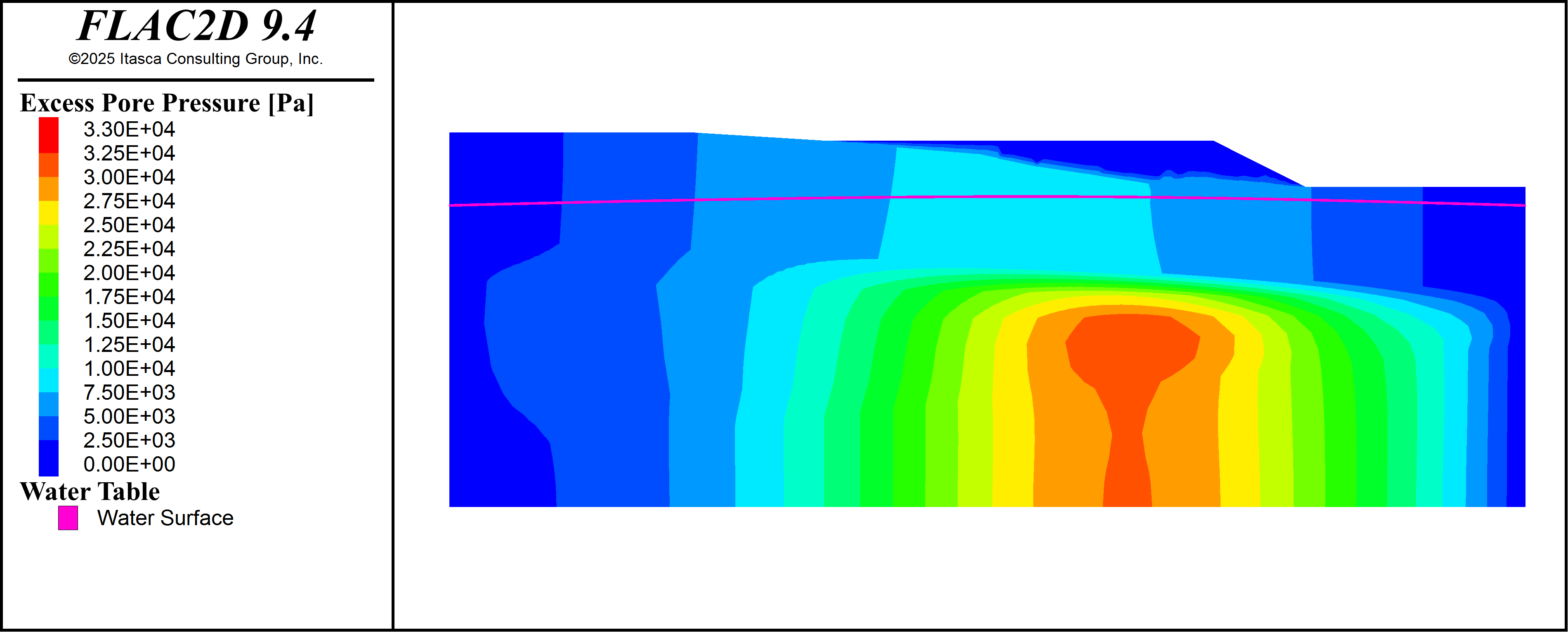
Figure 2: Excess pore pressure distribution after construction of the first lift (\(t=1\) day).
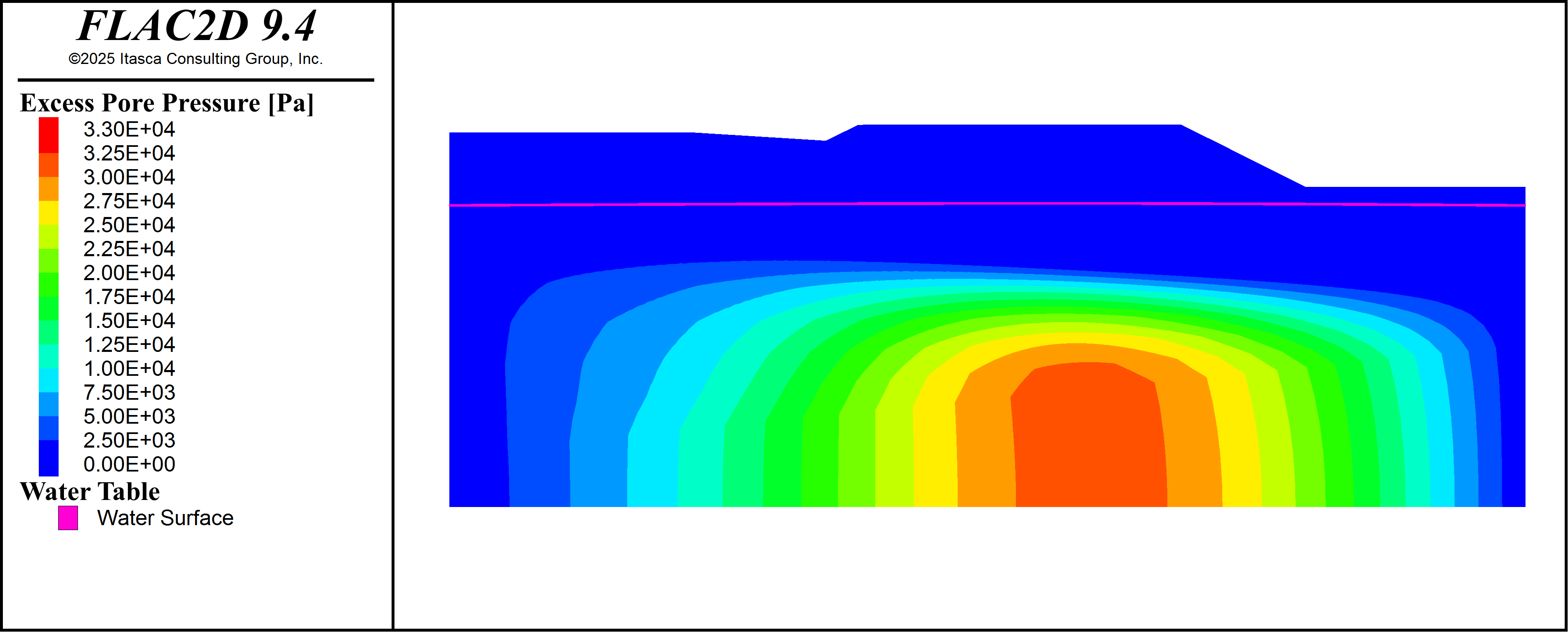
Figure 3: Excess pore pressure distribution after construction of the second lift (\(t=10\) days).
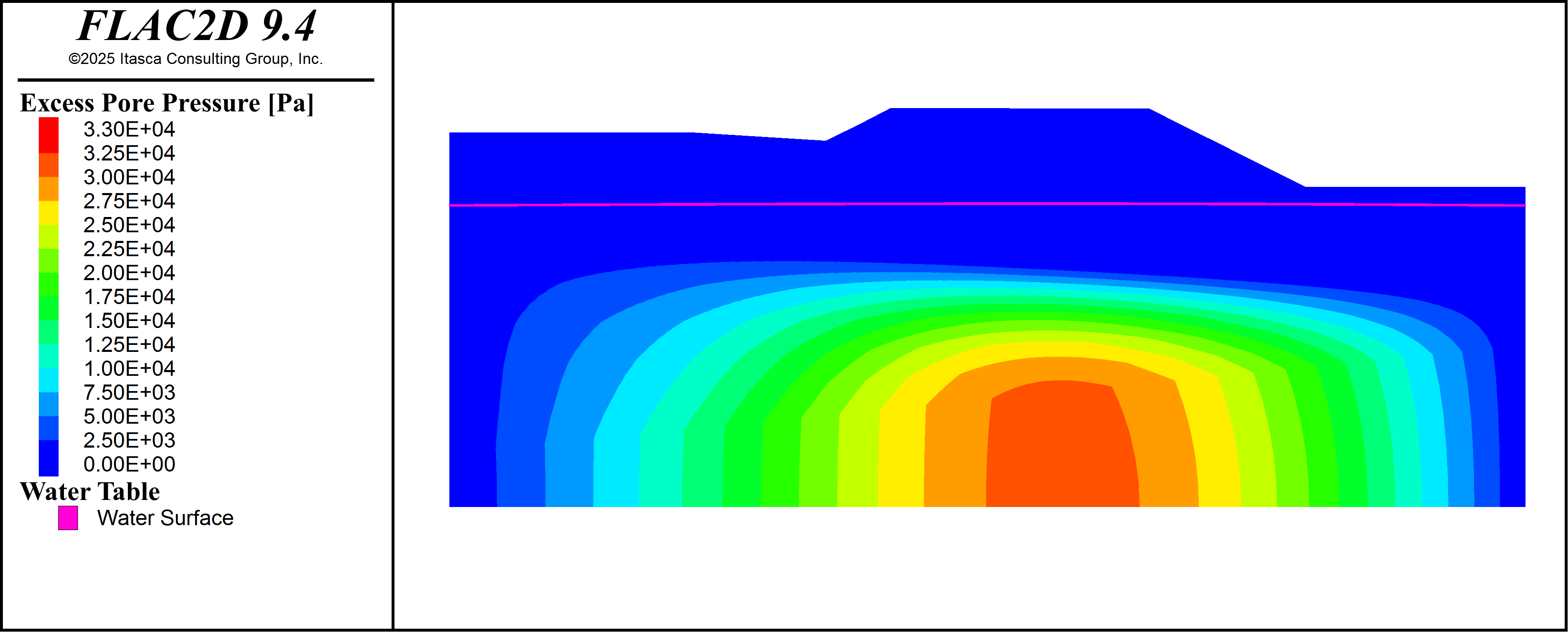
Figure 4: Excess pore pressure distribution after construction of the third lift (\(t=20\) days).

Figure 5: Excess pore pressure distribution after construction of the fourth lift (\(t=60\) days).
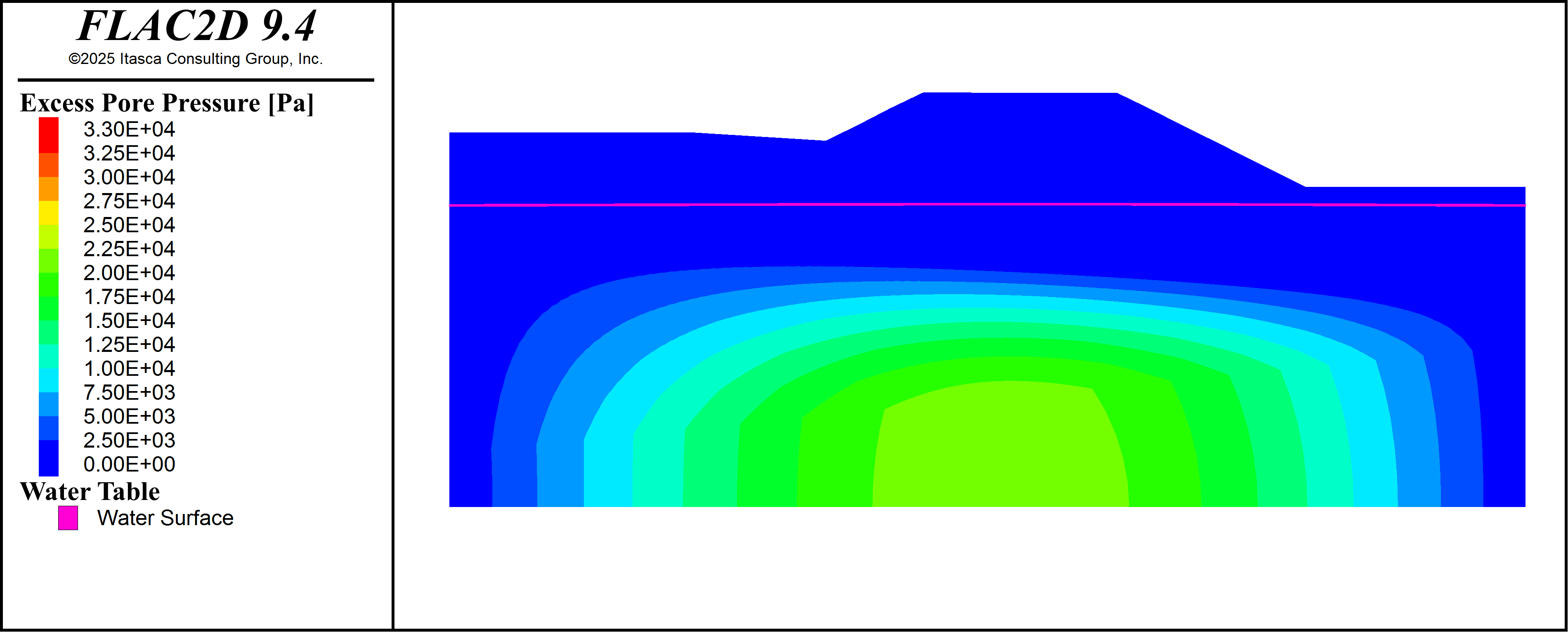
Figure 6: Excess pore pressure distribution after application of the traffic load (\(t=65\) days).
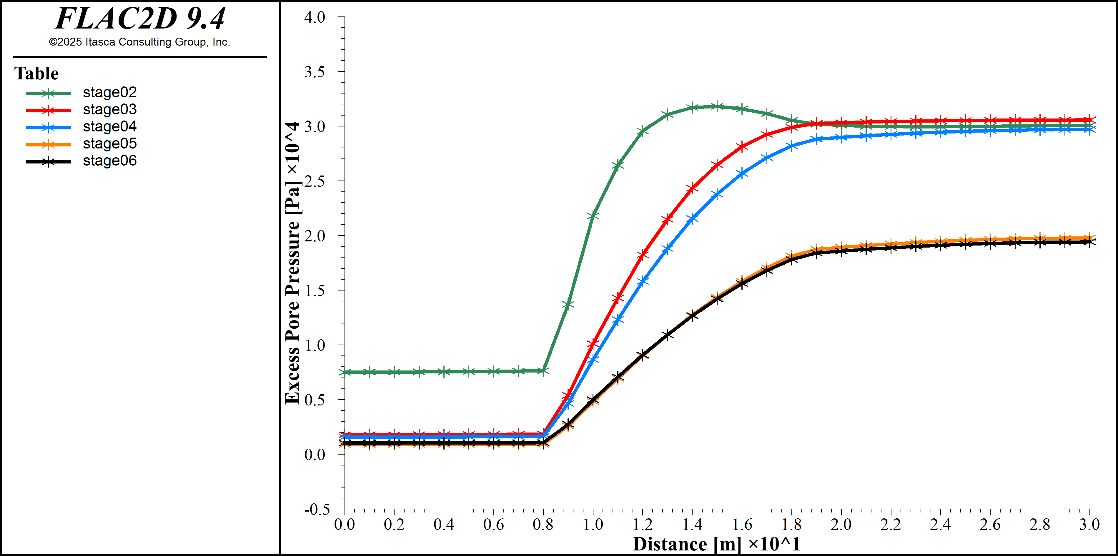
Figure 7: Excess pore pressure during the construction sequence. The x-axis represents the distance along a cut-line passing vertically from the base of the embankment to the base of the model.
Results - Settlement
The vertical displacement along a vertical line under the embankment and is stored in a table for plotting using a FISH function. Figure 8 shows the settlement during the construction sequence. The x-axis represents the distance along the cut-line with the base of the embankment at distance of 0 m and the base of the model at distance of 30 m. As with the excess pore pressure plots, the settlement profile for each stage could be generated with the Profile plot item, but in this example, the profiles were stored in tables using FISH so all stages could be plotted together.
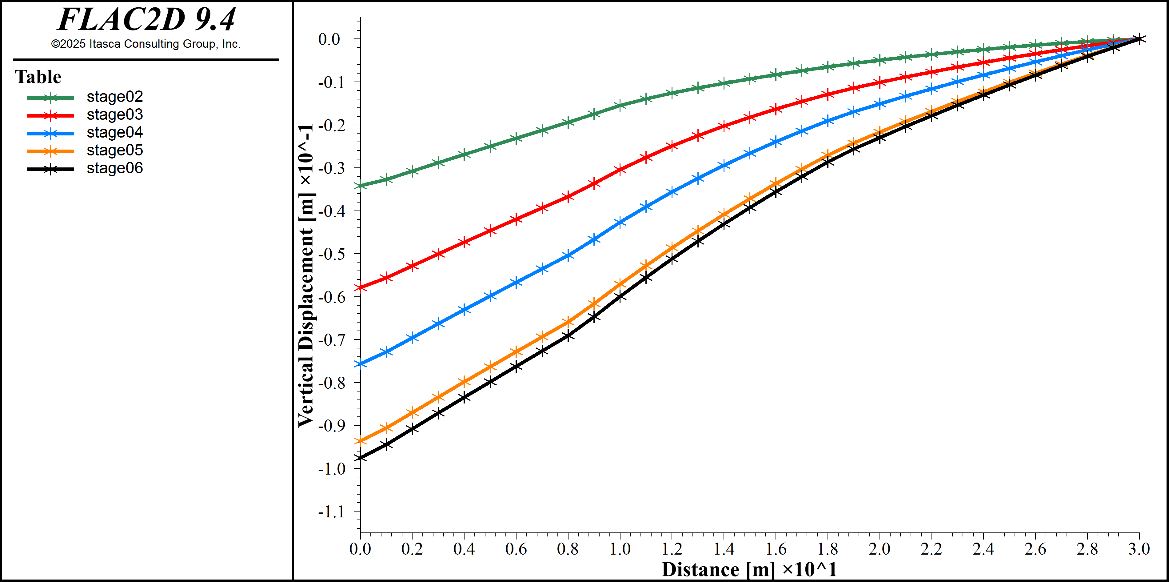
Figure 8: Vertical displacement during the construction sequence. The x-axis represents the distance along a cut-line passing vertically from the base of the embankment to the base of the model.
Data Files
consolidation.dat
; --------------------------------------- ;
;       MODEL SETUP and GEOMETRY          ;
; --------------------------------------- ;

model new

program call "mesh.dat" suppress

model configure fluid-flow
model gravity 9.81
model large-strain off

program call "functions.dat" suppress

; --------------------------------------- ;
;                STAGE 1                  ;
; --------------------------------------- ;

; Boundary Conditions
zone face skin
zone face apply velocity-x 0 range group 'West' or 'East'
zone face apply velocity 0 0 range group 'Bottom'

; Embankment - set properties, then null
zone cmodel assign elastic range group 'embankment'
zone property density 1334.86 bulk 11.11e6 shear 8.33e6 range group 'embankment'
zone null true keep-model range group 'embankment'

; Silty Sand I
zone cmodel assign mohr-coulomb range group 'Silty Sand I'
zone property density 1834.86 bulk 20.83e6 shear 9.62e6 range group 'Silty Sand I'
zone property cohesion 0.25e3 tension 0.25e3 friction 32 range group 'Silty Sand I'

; Silty Sand II
zone cmodel assign mohr-coulomb range group 'Silt Sand II'
zone property density 1834.86 bulk 11.11e6 shear 8.33e6 range group 'Silt Sand II'
zone property cohesion 0.1e3 friction 33 range group 'Silt Sand II'

; Silty Sand
zone cmodel assign mohr-coulomb range group 'Silty Sand'
zone property density 1834.86 bulk 13.89e6 shear 10.42e6 range group 'Silty Sand'
zone property cohesion 0.1e3 friction 35 range group 'Silty Sand'

; Initial Conditions
zone fluid-density 1e3
zone fluid property porosity 0.5
zone gridpoint pore-pressure head -12

zone effective-stress-cutoff 0
zone initialize-stresses ratio 0.5

; Solve to static equilibrium
zone nodal-mixed-discretization off
model solve-static convergence 0.01

; store "initial" pore pressure due to gravity
[gp.extra(::gp.list, 1) ::= 9810 * (-12 - gp.pos(::gp.list)->y)]
[save_settlement('stage1-uy')]
[save_excess_pp('stage1-pp')]
model save "stage01"

; --------------------------------------- ;
;                STAGE 2                  ;
; --------------------------------------- ;

; Undrained response
zone gridpoint initialize displacement 0 0
zone null false range group 'Layer1'
zone gridpoint initialize head -12 range group 'Layer1'
zone initialize-stresses ratio 0.8 range group 'Layer1'

zone fluid modulus-automatic

zone face apply head -12 range group 'West' or 'East'
zone fluid property pore-pressure-generation on ...
    range group "embankment" not

model solve-static convergence 1

; Consolidation
zone fluid property hydraulic-conductivity 5e-6 range group 'Silty Sand I'
zone fluid property hydraulic-conductivity 2e-8 range group 'Silt Sand II'
zone fluid property hydraulic-conductivity 1e-7 range group 'Silty Sand'
zone fluid cmodel assign inactive range group 'Layer1'

zone fluid modulus-scale range group 'embankment' not
zone fluid property pore-pressure-generation off

zone fluid implicit on
zone fluid timestep fix 864
zone fluid implicit servo off
zone fluid implicit solver pcg

model solve-fluid-decoupled time 86400 convergence 1 stages 5
[save_settlement('stage2-uy')]
[gp.extra(::gp.list,2) ::= gp.pp(::gp.list) - gp.extra(::gp.list,1)]
[save_excess_pp('stage2-pp')]
model save "stage02"

; --------------------------------------- ;
;                STAGE 3                  ;
; --------------------------------------- ;

; Undrained response
zone null false range group 'Layer2'
zone gridpoint initialize head -12 range group 'Layer2'
zone initialize-stresses ratio 0.8 range group 'Layer2'

zone fluid modulus-automatic

zone fluid property pore-pressure-generation on ...
    range group "embankment" not

model solve-static convergence 1

; Consolidation
zone fluid cmodel assign inactive range group 'Layer2'
zone fluid modulus-scale range group 'embankment' not
zone fluid property pore-pressure-generation off

model solve-fluid-decoupled time [86400*9] convergence 1 stages 5
[save_settlement('stage3-uy')]
[gp.extra(::gp.list,2) ::= gp.pp(::gp.list) - gp.extra(::gp.list,1)]
[save_excess_pp('stage3-pp')]
model save "stage03"

; --------------------------------------- ;
;                STAGE 4                  ;
; --------------------------------------- ;

; Undrained response
zone null false range group 'Layer3'
zone gridpoint initialize head -12 range group 'Layer3'
zone initialize-stresses ratio 0.8 range group 'Layer3'

zone fluid modulus-automatic

zone fluid property pore-pressure-generation on ...
    range group "embankment" not

model solve-static convergence 1

; Consolidation
zone fluid cmodel assign inactive range group 'Layer3'
zone fluid modulus-scale range group 'embankment' not
zone fluid property pore-pressure-generation off

model solve-fluid-decoupled time [86400*10] convergence 1 stages 5
[save_settlement('stage4-uy')]
[gp.extra(::gp.list,2) ::= gp.pp(::gp.list) - gp.extra(::gp.list,1)]
[save_excess_pp('stage4-pp')]
model save "stage04"

; --------------------------------------- ;
;                STAGE 5                  ;
; --------------------------------------- ;

; Undrained response
zone null false range group 'Layer4'
zone gridpoint initialize head -12 range group 'Layer4'
zone initialize-stresses ratio 0.8 range group 'Layer4'

zone fluid modulus-automatic

zone fluid property pore-pressure-generation on ...
    range group "embankment" not

model solve-static convergence 1

; Consolidation
zone fluid cmodel assign inactive range group 'Layer4'
zone fluid modulus-scale range group 'embankment' not
zone fluid property pore-pressure-generation off

model solve-fluid-decoupled time [86400*40] convergence 1 stages 5
[save_settlement('stage5-uy')]
[gp.extra(::gp.list,2) ::= gp.pp(::gp.list) - gp.extra(::gp.list,1)]
[save_excess_pp('stage5-pp')]
model save "stage05"

; --------------------------------------- ;
;                STAGE 6                  ;
; --------------------------------------- ;

; Undrained response
zone face apply stress-normal -10e3 range position-y -1.50949 tolerance 1e-1

zone fluid modulus-automatic

zone fluid property pore-pressure-generation on ...
    range group "embankment" not

model solve-static convergence 1

; Consolidation
zone fluid modulus-scale range group 'embankment' not
zone fluid property pore-pressure-generation off

model solve-fluid-decoupled time [86400*5] convergence 1 stages 5
[save_settlement('stage8-uy')]
[gp.extra(::gp.list,2) ::= gp.pp(::gp.list) - gp.extra(::gp.list,1)]
[save_excess_pp('stage8-pp')]
model save 'stage08'
functions.dat
fish define save_settlement(name)
    zone.field.name = 'displacement-y'
    local result = 0.0
    local yvalues = list.range(-40, -10, 1)
    local k = 1
    loop foreach local yv yvalues
        result = zone.field.get(vector(65, yv))
        table.x(name,k) = math.abs(yv - list.max(yvalues))
        table.y(name,k) = result
        k += 1
    endloop
end

fish define save_excess_pp(name)
    zone.field.extra = 2
    zone.field.name = 'extra'
    local result = 0.0
    local yvalues = list.range(-40, -10, 1)
    local k = 1
    loop foreach local yv yvalues
        result = zone.field.get(vector(65, yv))
        table.x(name,k) = math.abs(yv - list.max(yvalues))
        table.y(name,k) = result
        k += 1
    endloop
end
⇐ Deformation Caused by Filling of a Caisson (FLAC2D) | Embankment Consolidation (Soft-Soil) (FLAC2D) ⇒
| Was this helpful? ... | Itasca Software © 2024, Itasca | Updated: Jun 07, 2025 |
