Embankment Consolidation (Soft-Soil) (FLAC2D)

Problem Statement

Note

To view this project in FLAC2D, use the menu command Help ‣ Examples…. Choose “Embankment Consolidation (Soft-Soil)” and select “EmbankmentConsolidationSS.prj” to load. The project’s main data files are shown at the end of this example.

This example builds upon the Mohr-Coulomb embankment consolidation example by modeling the soil layers with effective stress-dependent stiffness, a volumetric hardening cap, and void ratio dependent conductivity, something more representative of soft soils compared to the Mohr-Coulomb model. This example also extends the staged construction sequence from the previously mentioned example to include sub-steps within each constructed lift. The embankment lift density is incremented from a small multiplier to the full value over these sub-steps to ensure solution convergence with highly nonlinear material behavior. The main idea of the staged construction sequence, however, remains the same: honor the physical construction time that is needed to construct each lift without causing large excess pore pressures in the model.

The embankment is constructed in two lifts (each 2 meters in height) over a duration of 58 days, during which pore pressure dissipation and soil consolidation takes place. The full construction sequence is given in Table 1 which includes alternating steps of construction and excess pore pressure drainage. Due to symmetry at the center of the embankment, only the right half is modeled. The model initially contains the two embankment layers but they are nulled prior to gravity initialization. The null zones are considered not present for most purposes during calculations or plotting. Each embankment lift is un-nulled at the time of construction, providing and additional load due to the weight of each lift.

Table 1: Embankment Construction Sequence

Sequence Step	Description	Duration (days)	Solution Type
01	Initilization	0	Mechanical
02	Construct lift 1	2	Fluid-Mechanical
02	Pore pressure dissipation	30	Fluid-Mechanical
03	Construct lift 2	1	Fluid-Mechanical
04	Pore pressure dissipation	25	Fluid-Mechanical

The model is constructed in Sketch and groups are assigned to the different soil layers. Three soil layers are present in the model (from surface to depth): peat, clay, and dense sand. The thickness of these layers are 3, 3, and 4 meters, respectively. The embankment is composed of loose sand. The model geometry and soil layers are shown in Figure 1.

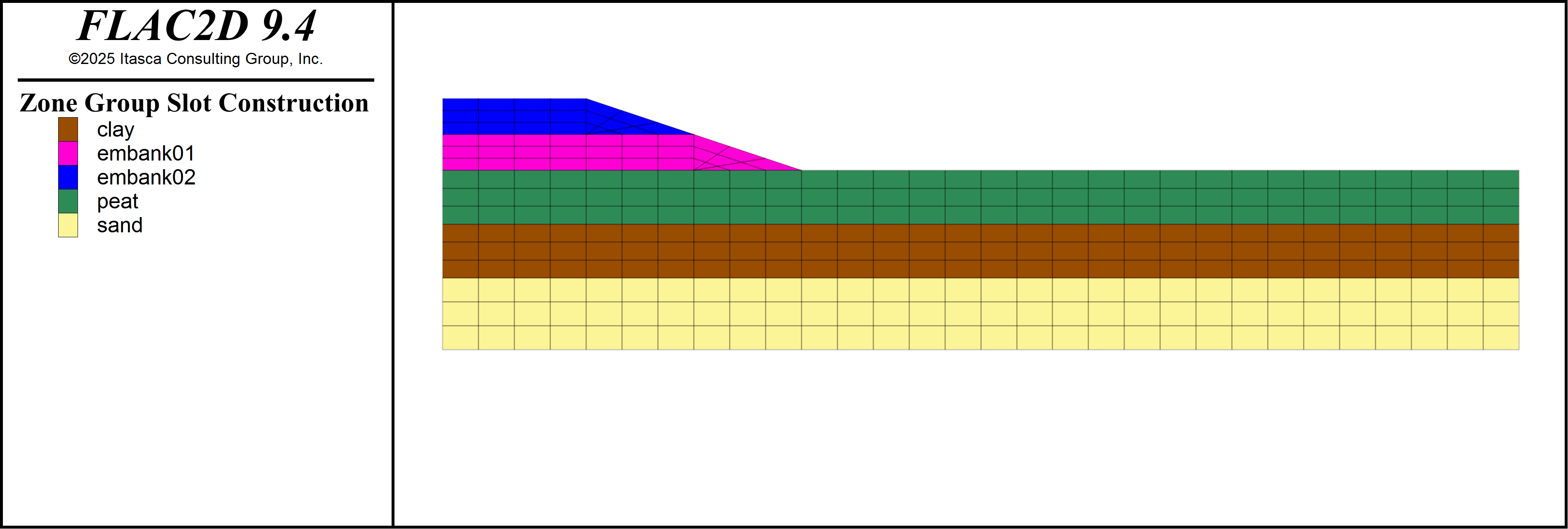
Figure 1: Model geometry, soil layers, and embankment lifts.

The peat and clay layers are modeled with a Soft-Soil constitutive law. The dense sand layer is modeled with a Plastic-Hardening constitutive law, and the embankment is modeled with a Mohr-Coulomb constitutive law. The embankment is considered impermeable in the model so that excess pore pressures due to embankment loading must dissipate through the dense sand layer. The material properties for the peat and clay layers are given in Table 2. Note that these layers are the only ones allowed to generate excess pore pressure in the model.

Table 2: Material Properties for Soft-Soil materials

Property	Peat	Clay
Dry density \(\rho\) (kg/m3)	815.5	1530
modified swelling index \(\kappa^*\)	0.03	0.01
modified compression index \(\lambda^*\)	0.15	0.05
poisson’s ratio \(\nu\)	0.15	0.15
initial void ratio \(e_0\)	2.0	1.0
friction angle \(\phi\) (Deg)	23	25
cohesion \(c\) (kPa)	2	1
over consolidation ratio \(OCR\)	1.0	1.0
horizontal conductivity \(k_h\) (m/day)	1.0	0.047
vertical conductivity \(k_v\) (m/day)	0.05	0.047
consolidation coefficeint \(C_v\) (m2/day)	1.3	6.5

Loosely Coupled Fluid-Mechanical Approach

The fluid-mechanical coupling approach used in this example is similar to the one used in the Mohr-Coulomb embankment consolidation example, but with a few changes to the drained step to handle the elastoplastic K₀ effective stress path taken during consolidation for normally consolidated soft soils. Familiarization with the previously mentioned example is recommended prior to this one. The loosely coupled approach performs an undrained step with the “true” fluid modulus. The command zone fluid modulus-automatic is used to scale the fluid modulus and speed up the calculation. The command zone fluid property pore-pressure-generation on is used to force generation of pore pressures caused by deformation. The undrained step is then followed by a drained step using the commands zone fluid property consolidation-coefficient and model solve-fluid-decoupled. The consolidation coefficient is the recommended method of setting the “scaled” fluid modulus for normally consolidated soils with effective stress-dependent stiffness. This is because the command zone fluid modulus-scale approximates confined elastic compressibility, defined by a stress path of \(\Delta \sigma^\prime_h = \nu /\left( 1-\nu \right) \cdot \Delta \sigma^\prime_v\) instead of \(\Delta \sigma^\prime_h = K_0 \cdot \Delta \sigma^\prime_v\). Typically, in the geotechnical engineering field, the consolidation coefficient is known, either from oedometer tests on undisturbed soil samples in the laboratory or piezocone penetration tests on in-situ soils. The consolidation coefficient, however, can be estimated with:

(1)\[C_v = \frac{k_v}{\gamma_w m_v}\]

where \(C_v\) is the consolidation coefficient, \(k_v\) is the vertical hydraulic conductivity, \(\gamma_w\) is the unit weight of water, and \(m_v\) is the confined skeleton compressibility.

In practice, the consolidation coefficient remains mostly constant during consolidation as both the confined skeleton compressibility and hydraulic conductivity decrease with increase of effective stress. The net result is that \(C_v\) remains mostly constant. For example, a common choice for hydraulic conductivity is:

(2)\[k_v = k_{v0} \cdot 10^{\Delta e / \beta}\]

(3)\[\frac{1}{m_v} = \frac{\partial \sigma^\prime_{v}}{\partial \varepsilon_v}\]

where \(k_{v0}\) is the initial conductivity, \(\Delta e\) is change of void ratio, and \(\beta\) is a fitting parameter. This is the approach taken in this model, i.e., the consolidation coefficeint is not updated during consolidation.

Staged Construction Sequence

As previously mentioned, the embankment is constructed in two lifts over a period of 58 days. The construction of each lift if divided into five sub-steps. Prior to the construction sequence, the the embankment lift is un-nulled with zone null set to false. One sub-step includes the following procedure:

1. Assign a partial density to the embankment lift with zone property density. For five sub-steps, the density multiplier is set to 0.2, 0.4, 0.6, 0.8, and 1.0.

2. Horizontal stress is initialized in the embankment lift to K₀ conditions with zone initialize-stresses.

3. The “true” fluid stiffness is set using zone fluid modulus-automatic. (This assumes the fluid is essentially incompressible relative to the soil and therefore sets the fluid modulus to be 20x stiffer than the soil stiffness). Note that the biot modulus is set to 0 before executing this command because the automatically calcuated modulus will not be used if the existing modulus is lower (and non-zero).

4. Pore pressure generation is activated in the soil layers with zone fluid property pore-pressure-generation.

5. The model is solved to undrained static equilibrium with model solve-static. This step involves zero time, i.e., it is considered the instantaneous response.

6. The fluid stiffness is scaled to account for skeleton compressibility with zone fluid property consolidation-coefficient.

7. The model is solved for a period of time to allow for pore pressure dissipation and consolidation with model solve-fluid-decoupled. The time in this step is physical and represents the construction time. This example uses a total time of 2 days for the first lift and 1 day for the second lift. Hence, the physical time in this step also sub-divided into five increments, i.e., this step is solved five times for 0.4 days to reach the total 2 days for the first lift.

This process is repeated five times for each lift until all lifts have been constructed. Additonal fluid drainge occurs between construction of the two lifts.

Model Initialization

The first step in the model is to initialize the in-situ stresses, pore pressures, and the volumetric yield surface for the soft-soil layers. This is accomplished by first setting the nonlinear materials to a Mohr-Coulomb constitutive model, applying a hydrostatic pore pressure gradient with zone gridpoint initialize head, initializing the horizontal effective stresses (both in and out of plane in 2D) to K₀ conditions with zone initialize-stresses ratio, and solving to static equilibrium. Once the in-situ stresses are initialized, the constitutive models are switched to nonlinear and the model is solved once again to static equilibrium. The in-situ state is shown on Figure 2 to Figure 5.

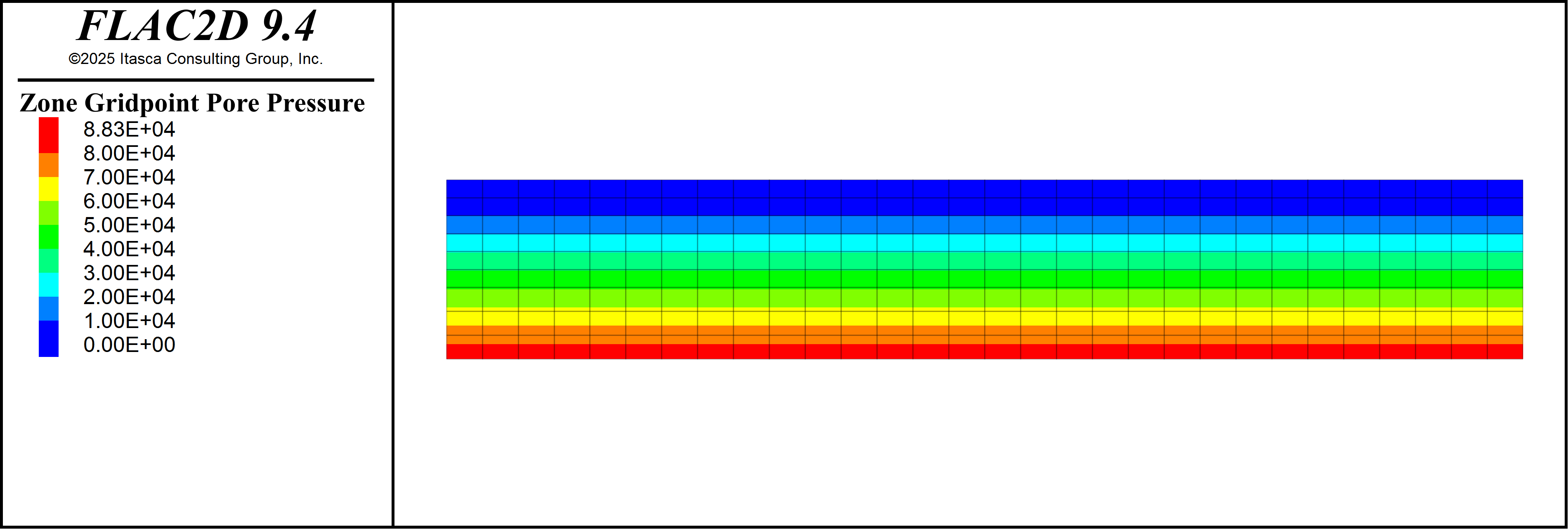
Figure 2: Initial pore pressure distribution.

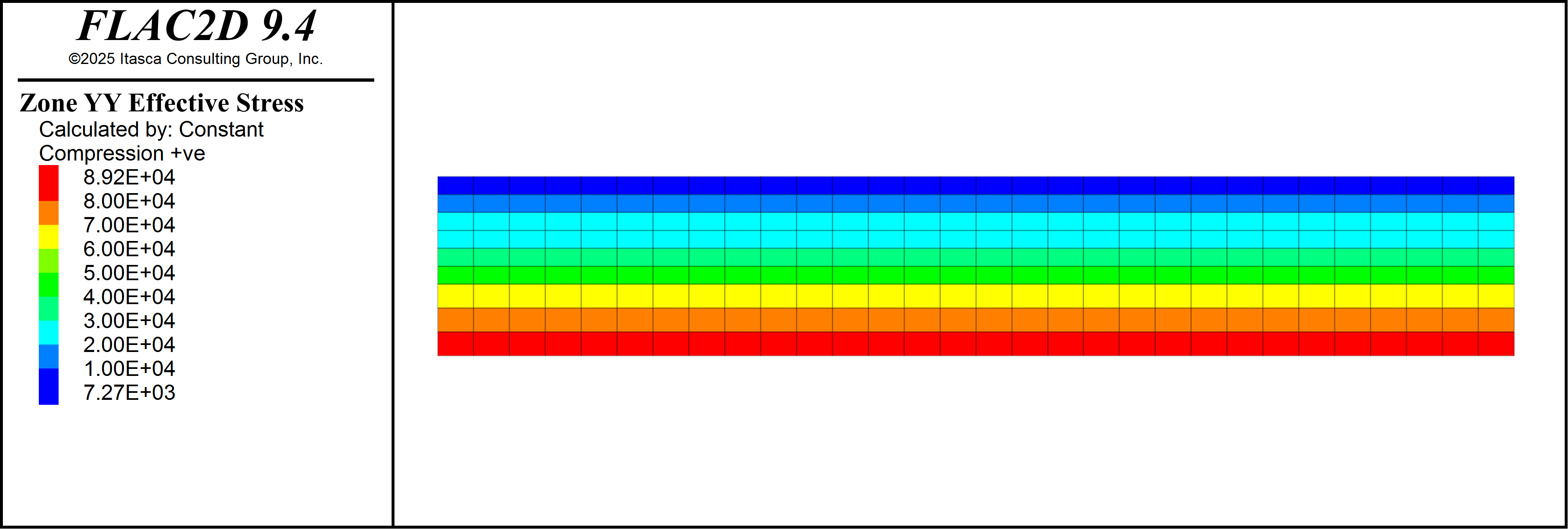
Figure 3: Initial vertical effective stress.

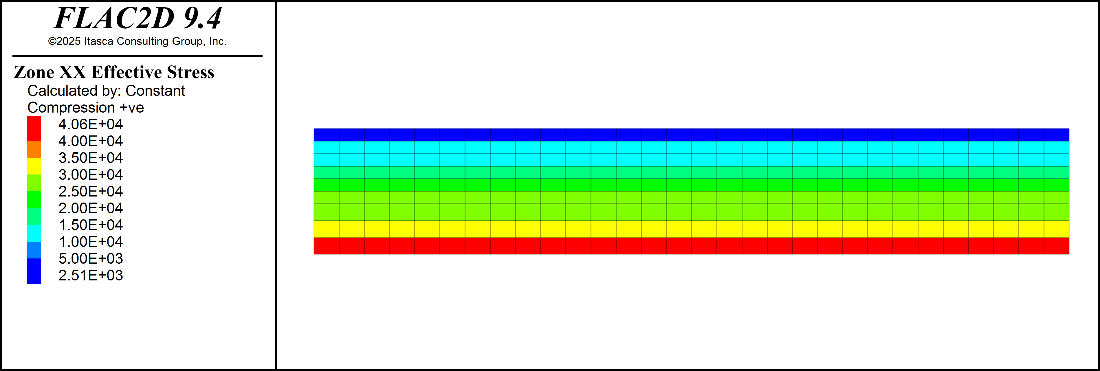
Figure 4: Initial horizontal effective stress.

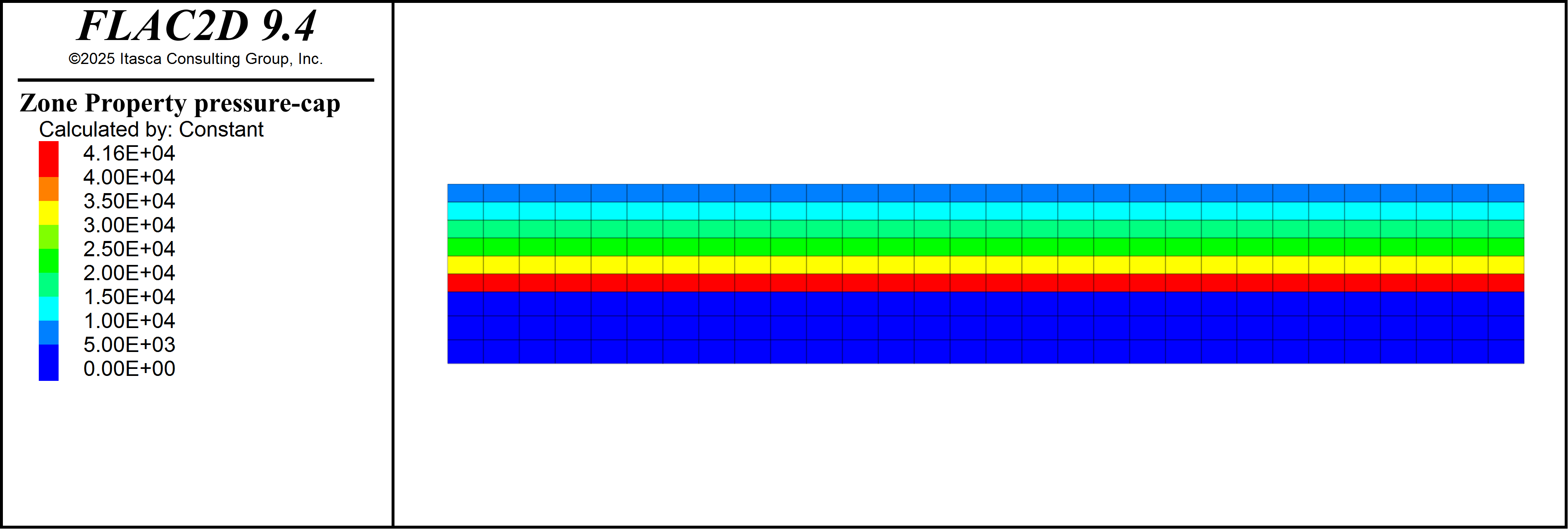
Figure 5: Initial volumetric yield cap for soft-soil materials.

Results - Excess Pore Pressure

Excess pore pressure (current pressure minus initial hydrostatic pressure) is calculated in the same way as Mohr-Coulomb embankment consolidation example, and will not be repeated here. The excess pore pressure distribution immediately after construction of each embankment lift is shown below. Note that 30 days of pore pressure dissipation occcurs between Figure 6 and Figure 7.

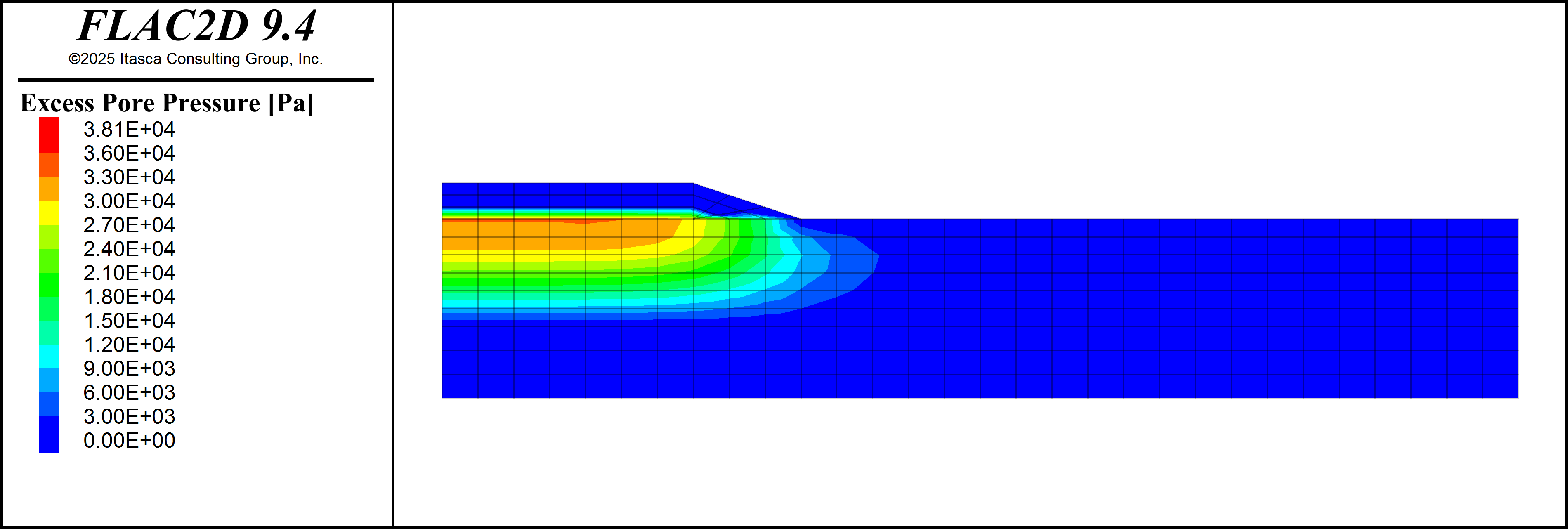
Figure 6: Excess pore pressure immediately after construction of the first lift.

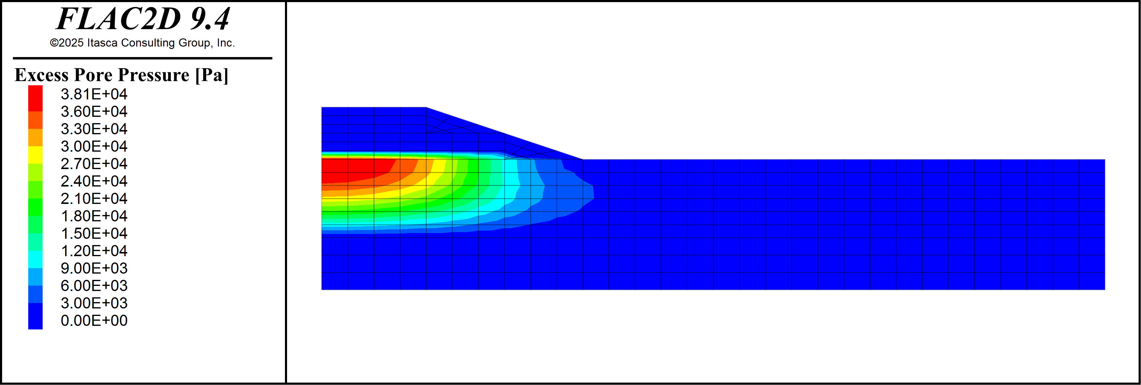
Figure 7: Excess pore pressure immediately after construction of the second lift.

Results - Total and Effective Stresss

Figure 8 shows the total and effective vertical stress response during the construction periods (0-2 days, 32-33 days) and during the pressure dissipation periods (2-32 days, 33-58 days). The history location is at the center of the embankment and between the peat and clay layers. Total vertical stress remains constant during pore pressure dissipation periods while effective stress increases. Note that the figure below utilizes geomechanics sign convention for total and effective horizontal stress (compressive stress changes positive) in order to visualize together with pore pressure.

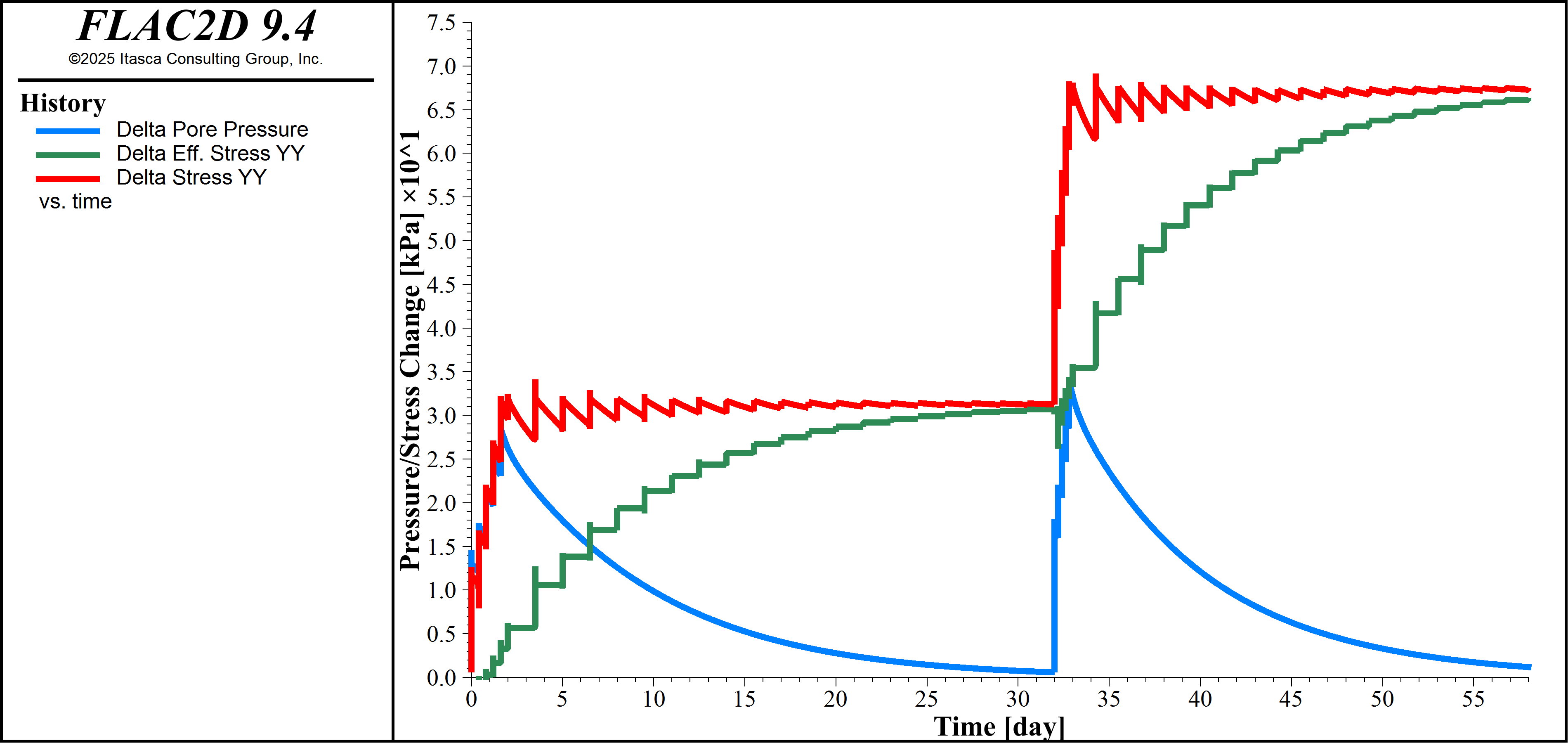
Figure 8: Pore pressure, vertical effective stress, and vertical total stress history at a point between the peat and clay layers and at the center of the embankment.

Data Files

initialize.dat

; ---------------------------------- ;
;           Initialization           ;
; ---------------------------------- ;

; Mechanical boundary conditions
zone face skin
zone face apply velocity-x 0 range group "East" or "West"
zone face apply velocity 0 0 range group "Bottom"

; Linear material model for stress initialization
zone cmodel assign mohr-coulomb

zone property density 1.3e3 friction 30.0 ...
    cohesion 2e3 young 25e6 poisson 0.2 ...
    range group "embank01" or "embank02"

zone property density 815.5 friction 23.0 ...
    cohesion 2e3 young 50e3 poisson 0.15 ...
    range group "peat"

zone property density 1529.05 friction 25.0 ...
    cohesion 1e3 young 50e3 poisson 0.15 ...
    range group "clay"

zone property density 1732.93 friction 33.0 ...
    cohesion 0 dilation 3 young 50e3 poisson 0.15 ...
    range group "sand"
    
zone fluid property porosity 0.333 range group "embank01"

zone fluid property porosity 0.6667 range group "peat"

zone fluid property porosity 0.5000 range group "clay"

zone fluid property porosity 0.3333 range group "sand"
    
; Null embankment for initialization
zone null true keep-model range group "embank01" or "embank02"

; Initialize pore pressure
zone fluid-density 1.0e3
zone gridpoint initialize head -1

; Fluid flow properties
zone fluid property hydraulic-conductivity-tensor ...
    1.157e-6 5.787e-7 range group "peat"

zone fluid property hydraulic-conductivity-tensor ...
    5.5e-7 5.5e-7 range group "clay"
    
zone fluid property hydraulic-conductivity-tensor ...
    8.25e-5 8.25e-5 range group "sand"

; Initialize effective stresses with K0 = 1 - sin(phi)
zone initialize-stresses ratio [1.0-math.sin(33*math.pi/180)] ...
    range group "sand"
zone initialize-stresses ratio [1.0-math.sin(25*math.pi/180)] ...
    range group "clay"
zone initialize-stresses ratio [1.0-math.sin(23*math.pi/180)] ...
    range group "peat"

; Solve mechancial only
model solve-static convergence 1

; Switch to nonlinear material models
zone cmodel assign soft-soil range group "peat" or "clay"
zone cmodel assign plastic-hardening range group "sand"

zone property kappa-modified 0.03 lambda-modified 0.15 ...
    void-initial 2.0 cohesion 2e3 friction 23 ...
    range group "peat"
    
zone property kappa-modified 0.01 lambda-modified 0.05 ...
    void-initial 1.0 cohesion 1e3 friction 25 ...
    range group "clay"
   
zone property exponent 0.5 stiffness-50-reference 35e6 ...
    stiffness-oedometer-reference 35e6 ...
    stiffness-ur-reference 105e6 void-initial 0.5 ...
    pressure-reference 1e5 cohesion 0 dilation 3 ...
    friction 33 over-consolidation-ratio 1.0 ...
    range group "sand"

; Initialize the yield surface
[initialize_stress()]

; Solve mechancial only
model solve-static convergence 1
[initialize_extra()]
model save "init.sav"

consolidation.dat

; ---------------------------------- ;
;        Construct first lift        ;
; ---------------------------------- ;

model restore "init.sav"
zone gridpoint initialize displacement 0 0

; Activate the first embankment stage
zone null false range group "embank01" 
zone fluid cmodel assign inactive range group "embank01"
zone gridpoint initialize head -1 range group "embank01"

; Fluid boundary conditions
zone gridpoint fix pore-pressure 0 gradient 0 -9810 ... 
    origin 0 -1 range group "Bottom" or "East" or "sand"
zone gridpoint fix head -1 range position-x 20 1e99 position-y 0

; Implicit fluid solver
zone fluid implicit on
zone fluid timestep maximum 864
zone fluid implicit servo on

; Solve construction sequence for t = 2 days

; histories
[zone = zone.near(0, -3.0)]
fish history name "press" [(zone.pp(zone) - zone.extra(zone, 4))/1e3]
fish history name "stress" [-(zone.stress(zone)->yy - zone.extra(zone, 2))/1e3]
fish history name "stress_eff" [-(zone.stress.effective(zone)->yy - zone.extra(zone, 3))/1e3]
fish history name "time" [fluid.time.total / 8.64e4]
 
[staged_construction(n=5, days=2, group="embank01")]
model save "stage01.sav"

; Conoslidate for t = 30 days
model solve-fluid-decoupled time [86400*30] stages 20
model save "stage02.sav"

; ---------------------------------- ;
;       Construct second lift        ;
; ---------------------------------- ;

; Activate the second embankment stage
zone null false range group "embank02"
zone fluid cmodel assign inactive range group "embank02"
zone gridpoint initialize head -1 range group "embank02"

; Solve construction sequence for t = 1 days
[staged_construction(n=5, days=1, group="embank02")]
model save "stage03.sav"

; Conoslidate for t = 25 days
model solve-fluid-decoupled time [86400*25] stages 20
model save "stage04.sav"

functions.dat

; ---------------------------------- ;
;           FISH Functions           ;
; ---------------------------------- ;

fish define initialize_stress
    local zones = zone.list( zone.model(::zone.list) != 'null' )
    local pp = math.max(::zone.pp(::zones), 0.0) ; Cutoff = 0.0
    local prin = tensor.prin(::zone.stress(::zones))
    zone.prop(::zones,'stress-1-effective') ::= prin->x + pp
    zone.prop(::zones,'stress-2-effective') ::= prin->y + pp
    zone.prop(::zones,'stress-3-effective') ::= prin->z + pp
end

fish define initialize_extra
    gp.extra(::gp.list, 1) ::= 9810 * (-1 - gp.pos(::gp.list)->y)
    zone.extra(::zone.list, 2) ::= zone.stress(::zone.list)->yy
    zone.extra(::zone.list, 3) ::= zone.stress.effective(::zone.list)->yy
    zone.extra(::zone.list, 4) ::= 9810 * (-1 - zone.pos(::zone.list)->y)
end

fish define update_extra
    local p0 = gp.extra(::gp.list, 1)
    local sigma0 = zone.extra(::zone.list, 2)
    local sigma_e0 = zone.extra(::zone.list, 3)
    local pz0 = zone.extra(::zone.list, 4)

    gp.extra(::gp.list, 5) ::= gp.pp(::gp.list) - p0
    zone.extra(::zone.list, 6) ::= zone.stress(::zone.list)->yy - sigma0
    zone.extra(::zone.list, 7) ::= zone.stress.effective(::zone.list)->yy - sigma_e0
    zone.extra(::zone.list, 8) ::= zone.pp(::zone.list) - pz0
end

fish define staged_construction(n, days, group)
    local k = 1
    loop while k <= n
        command
            ; Ramp embankment density & initialize stress
            zone property density [1298*k/n] range group [group]
            zone initialize-stresses ratio 0.8 range group [group]
            
            ; Undrained response
            zone fluid property biot-modulus 0
            zone fluid modulus-automatic
            zone fluid property pore-pressure-generation on ...
                range group "peat" or "clay"
            model solve-static cycles 10000 convergence 1
            
            ; Consolidation
            zone fluid property biot-modulus 0  ; sand and embankment
            zone fluid property consolidation-coefficient [Cv_peat] ...
              range group 'peat'
            zone fluid property consolidation-coefficient [Cv_clay] ...
              range group 'clay'
            zone fluid property pore-pressure-generation off
            model solve-fluid-decoupled time [86400*days/n] stages 1

            [update_extra()]
        endcommand
        k += 1
    endloop
end