A Roadway Embankment with Surcharge Loads and Reinforcement (FLAC2D)
Problem Statement
Note
The project file for this example is available to be viewed/run in FLAC2D. [1]
The project’s main data file is shown at the end of this example.
This is an illustrative example of an embankment model with reinforcements and traffic loads. The original model was created in FLAC 8.1. Assumptions include that the slope and roadways exists as is, plane strain conditions are valid and long-term stability is related to drained soil conditions. A Mohr-Coulomb constitutive material model was used. Analyses focused on the use of the shear strength reduction (SSR) method to estimate the Factor of Safety (FoS) and plot FoS contours (i.e., a spatial distribution of FoS). Model properties (cohesion and friction) were incrementally decreased while monitoring displacements along the slope until equilibrium (slope is stable) was reached. Standard factor of safety analyses were performed for both drained and undrained cases, and ground reinforcement was added and factor of safety analysis values were compared for supported and unsupported cases.
The original FLAC 8.1 project is included with this example (embankment810.prj) to help understand the conversion process.
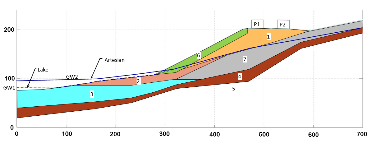
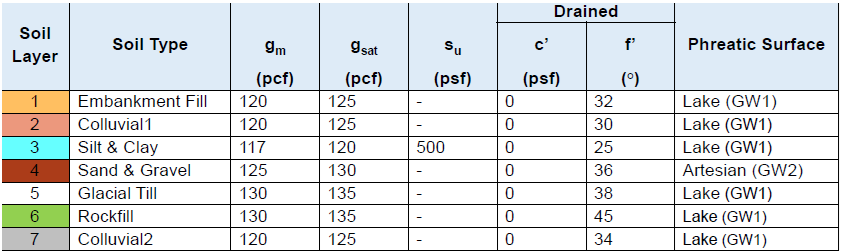
A cross-section of the embankment Figure 1 shows the soil layers, water tables and the locations of the traffic loads. Soil properties, water tables, and loads are provided in Figure 2
Figure 1: A cross section of the roadway embankment.
Figure 2: Embankment soil properties.
Model Geometry
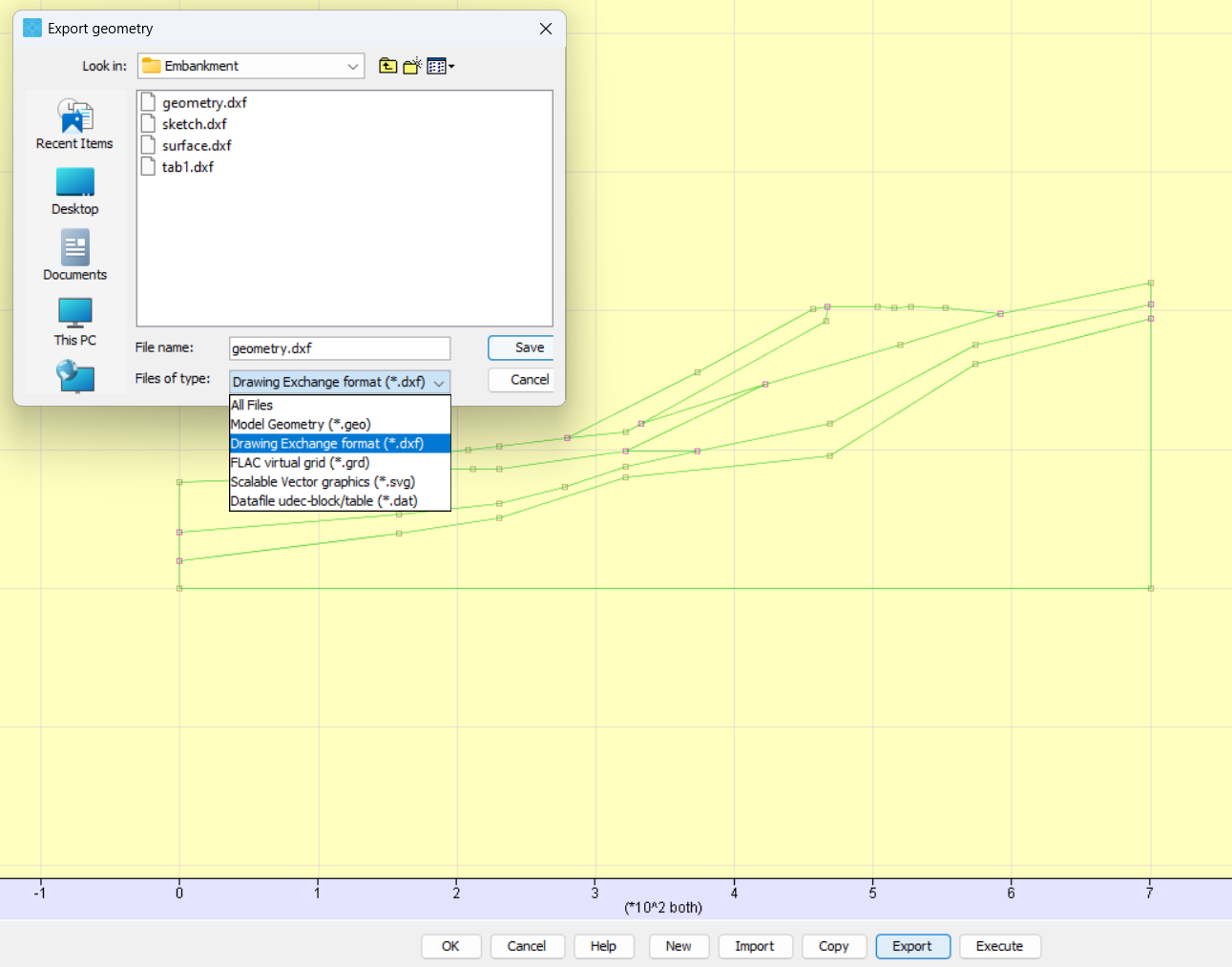
The model geometry in this example is exported from FLAC 8.1 as dxf file and then imported to FLAC2D Sketch workspace. This was done by opening FLAC 8.1 GUI (or v8.0,v7.0), going to Build/Sketch and selecting Export and Files of type as dxf, as shown in Figure 3.
Figure 3: Export sketch lines from FLAC as dxf file.
Start FLAC2D, the mesh for this analysis will be created in the Sketch workspace by following these steps:
First, go to File ‣ New ‣ Sketch Set, create a new sketch with a name.
Next, press the button Importbackgrounddata..., import the “sketch.dxf” file (the file we exported from FLAC 8.1) and then press the button Automaticallycreateedgesfrombackgroundgeometry, the sketch should appear as shown below.
Figure 4: Import sketch lines to FLAC2D sketch workspace.
And next use autosize () on the MeshTools pulldown () to set zone length to 4. Then use Meshallpolygons (), also on the “Mesh Tools” pulldown, to add zones to the model blocks. The model should appear as shown below:
Figure 5: Embankment final mesh.
Finally, Press the Createzones button () to create the zones.
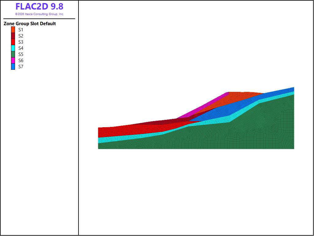
From the Model view in the workspace, select “Block 4”, and then select Assign a Group to the Selection… from the Commands pulldown and assign a group name “S6”, repeat this process until all groups are assigned with names, the model with different groups is shown below. Save the project and the model state.
Figure 6: The model view showing the different groups in the embankment.
Note that all of the sections of the model now have two group names. One that was automatically assigned by Sketch (Block=Block1, etc) and the groups that you just assigned (Default=S1 etc.). To more clearly see the groups that you assigned, you can change the Slot being plotted from Any to Default. Alternatively, you can make a new plot by going to File ‣ New ‣ Plot. Give the plot a name. Then click on the down arrow next to the BuildPlot tool button ( ), and select the Zone entry. Under the Attributes, change the Slot to Default and the model should appear as in Figure 7. Now it is a good idea to save the project File ‣ Save Project. When prompted, also save the state.
Figure 7: Embankment with different groups of layers.
Material Properties
We can use the Model view to assign constitutive models and the material properties, or create a datafile and write commands to it. From this point forward, data files are used to perform the analysis. An elastic constitutive model is initially assigned to all zones, all layers use the same bulk and shear moduli but different densities. We will switch to Mohr-Coulomb materials later and use actual material properties for Factor-of-Safety calculations. The commands are shown in the data file mat.dat.
model restore'group.sav'zone cmodel assign elastic; NOTE: stress units are psf, length units are feetzone property bulk=1.e6 shear=1.e6zone property density=3.727 range group 'S1'zone property density=3.727 range group 'S2'zone property density=3.634 range group 'S3'zone property density=3.882 range group 'S4'zone property density=4.037 range group 'S5'zone property density=4.037 range group 'S6'zone property density=3.727 range group 'S7'model save'mat.sav'
Setup Initial Stress and Pore-Pressure
This model does not require a fluid flow analysis, but we can configure fluid flow to enable calculation of saturated densities. In the original FLAC 8.1 example, a FISH function was used to set pore pressures and densities based on the depth of zones below water tables. In FLAC2D we can do the same thing with commands. Two water tables are used, one represents water level from the lake (table 10), the other one represents Artesian water (table 11). There are two ways to add tables, you can use the tableadd command to add the x- and y- values of the entry, or you can use the tableimport command to read table files created in FLAC 8.1. To export table files from FLAC 8.1, go to Utility/Table, from the table list, select the table number and then press Save button to save the file as a tab file. Please note the table format in FLAC 8.1 is a slightly different from FLAC2D, a zero for interval should be specified after the number of points on the second line of the table file.
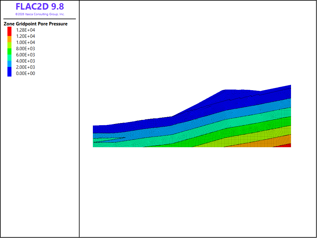
To accurately calculate material densities below the water table, we first configure the fluid flow with modelconfigurefluid-flow. Gravity is defined, the water tables are generated, porosities are assigned and the density of fluid is specified. To cause the material above the water table to become unsaturated (or partially saturated). A saturation model is specified with zonefluidunsaturated. In this example, we use the “cutoff” model, which means that any gridpoint with a pore pressure less than 0 is desaturated. Other models are available (see Saturated/Unsaturated Flow). By default, FLAC2D uses the saturated unit weight for all zones. To account for the effect of desaturation, use the command zonefluiddensity-saturatedoff. In this model, the effect of saturation on the results is negligible since the porosities are so low. Finally, the pore pressures (and saturations) are assigned with the zonegridpointpore-pressuretable command. The pore pressure contour plot is shown in Figure 8. Note that the contour lines can be made visible by expanding the Contour entry in the Attributes and checking the box for Isolines.
Figure 8: Embankment with pore pressure distribution and applied forces.
Static water pressure from the lake should be applied to the soil surfaces below the water table to account for the weight of the water. Traffic loads are also applied at the top surfaces. This can be performed by the following commands:
; lake loadzone face apply stress-normal -312 gradient 062.4... origin (0.0,76.0) range group 'top' position-x 073.4; traffic loadszone face apply stress-normal -360 range group 'top' position-x 475500zone face apply stress-normal -360 range group 'top' position-x 527552; Boundary conditions - roller on sides, fixed on bottomzone face apply velocity-x 0 range group 'East' or 'West'zone face apply velocity (0,0) range group 'Bottom'
The resulting applied forces are shown in Figure 8.
This model follows the standard boundary conditions: fixed degrees of freedom at the bottom and roller boundaries on the side surfaces. No fluid flow calcuation is required in this analysis, so the mechanical-only solution is obtained with the commands:
model fluid active offmodel solve convergence 1
It is also possible to solve for just the mechanical part with a single command (modelsolve-static), however, since we do not intend to do any fluid flow analysis for the rest of this model, it is useful to deactivate the fluid altogether at this point.
Factor-of-safety results under drained/undrained conditions
This stage includes four cases:
Case I: Factor-of-safety under drained condition.
Case II:Factor-of-safety under drained condition with reinforcements.
Case III: Factor-of-safety under undrained condition.
Case IV: Factor-of-safety under undrained condition with reinforcements.
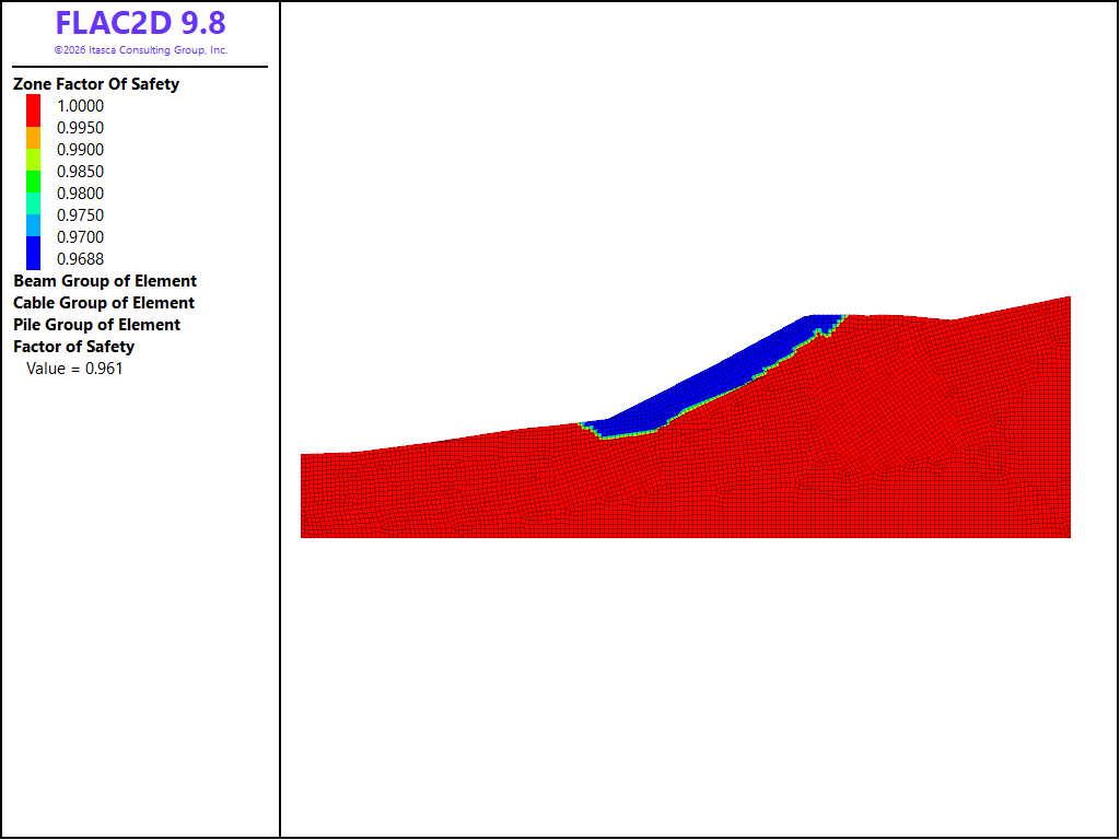
We first run the model under drained condition without any reinforcements. Before the factor-of-safety runs, the model should be re-initialized to zero displacements and velocities and be cleared of all yield states. We also switch the model from elastic to Mohr-Coulomb material and use the properties provided by the material table (Figure 2). The drained property is used for the Silt&Clay layer (S3). The factor-of-safety calculation is performed via command: modelfactor-of-safety. The factor of safety value and safety contour for drained case is shown in Figure 9. The calculated factor of safety is 0.957 (compare to 0.95 calculated by FLAC 8.1). This FOS map was created by plotting zones as described above, then choosing Color By ‣ Contour and Zone Value ‣ Factor of Safety. Then the Vel Limit was set to 0.001. See Factor of Safety Contours (FLAC2D) for more information about calculating and plotting factor of safety contours.
Figure 9: Factor of Safety contours for drained case.
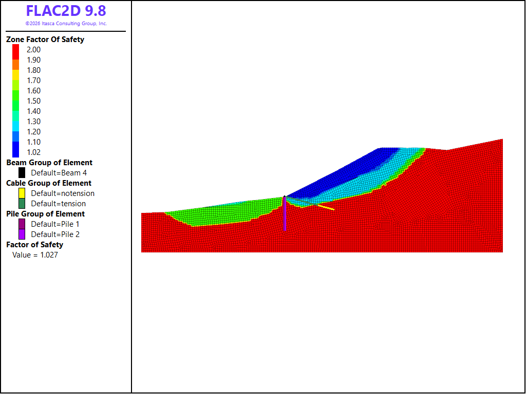
Two vertical drilled shafts are modeled by pile elements, and the concrete beam with grouted, tensioned anchors are modeled by beam elements and cable elements. A pretension force of 8.0E4 lbf is applied to the ungrouted cable to simulate the effect of the pressure grouting. (Note that the pretensioning parameter is also scaled automatically by the tieback spacing of 8 feet). The friction between the piles and the soil is assumed to be 25 degrees. The cable head is rigidly linked to the pile via the structurenodejoin command. Note that there must be coincident nodes to be able to join them (use the keyword snap when creating the cable elements to ensure that there are coincident nodes). The beam connects the two piles by using the existing nodes to create the beam. In this way, the structurenodejoin command is not required again (the model will not solve when three or more structural element nodes are joined together).
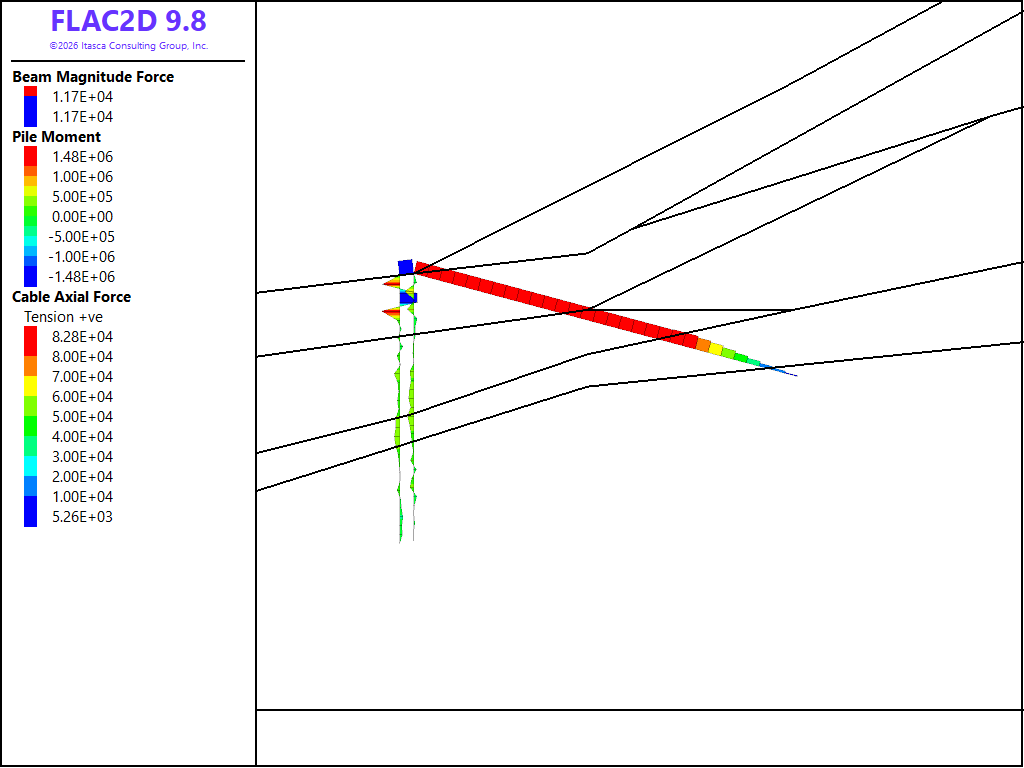
The factor of safety value and safety contour for drained condtions with reinforcements is shown in Figure 10. The FOS is calculated to be 1.03 (compared to 1.05 in FLAC 8.1). Moments in the piles and axial forces in the cables are shown in Figure 11.
Figure 10: Factor of Safety contours for drained case with reinforcements.
Figure 11: Forces and moments in the structural support for the drained case.
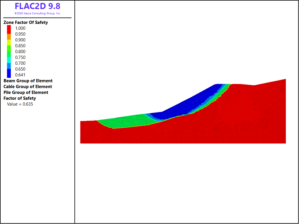
Unrained properties are used for the Silt&Clay layer (S3) in case III and the factor-of-safety calculation is performed again, results are shown in Figure 12. The model is less stable than the drained version as expected, showing a FOS of 0.63.
Figure 12: Factor of Safety contours for undrained case.
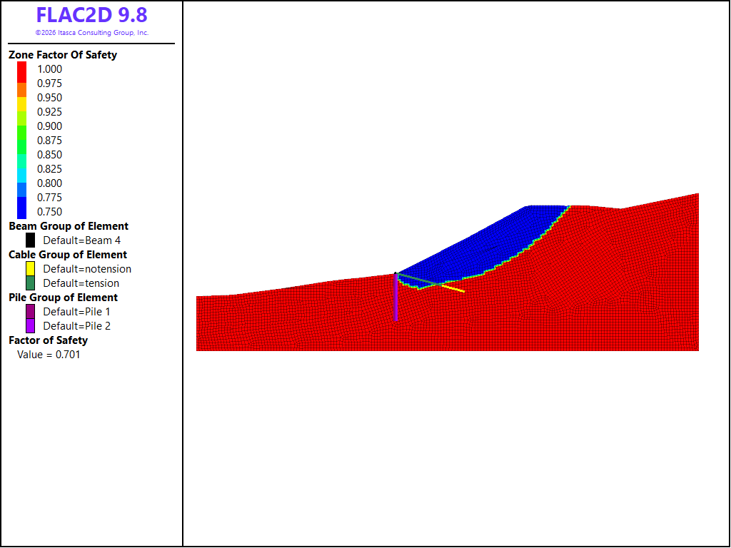
Reinforcements are installed (same as drained case), and the factor-of-safety calculation is performed. Results are shown in Figure 13. Note that for this model, the number of characteristic steps is manually specified for the FOS analysis. This is because the pretension in the cable and the weakness of the soil causes FLAC2D to fail to compute a characteristic number of steps. If no value is specified, then the default value of 200000 is used. If this specification of characteristic steps is omitted, you will obtain the same result for FOS, it will just take longer to solve.
Figure 13: Factor of Safety contours for undrained case with reinforcements.
Factor of Safety analyses using FLAC2D shows that without reinforcement, both the undrained and drained soil slope will fail (FoS of 0.63 and 0.96, respectively). The addition of drilled shafts and pre-tensioned grouted anchors near the slope toe stabilizes the slope, preventing the over-arching global failure mechanism for drained with a FoS of 1.03, however, the undrained slope will fail even with reinforcements, with a FoS of 0.69, that means more reinforcements are required to stabilize the slope.
Data Files
mat.dat
model restore'group.sav'zone cmodel assign elastic; NOTE: stress units are psf, length units are feetzone property bulk=1.e6 shear=1.e6zone property density=3.727 range group 'S1'zone property density=3.727 range group 'S2'zone property density=3.634 range group 'S3'zone property density=3.882 range group 'S4'zone property density=4.037 range group 'S5'zone property density=4.037 range group 'S6'zone property density=3.727 range group 'S7'model save'mat.sav'
pwp.dat
model restore'mat.sav'model large-strainoffmodel configure fluid-flowmodel gravity32.2; ft/s2table'10' add (0,81)(80,81)(139,90)(184,97)(208,100)(230,102)(279,108)...(322,120)(470,162)(574,180)(700,205)table'11' add (0,95)(158,99)(230,107)(322,120)(470,162)(574,180)(700,205); alternatively you can import tables exported from FLAC 8.1; a slight modification is required to the file format - see the example description;table '10' import 'table10';table '11' import 'table11'zone fluid property porosity 0.08009zone fluid property porosity 0.048054 range group 'S3'zone fluid-density1.94zone fluid unsaturated cutoffzone fluid property density-saturated false; assign pore pressures. The aquifer layer uses a different water tablezone gridpoint pore-pressure table '10'zone gridpoint pore-pressure table '11' range group 'S4'; identify boundarieszone face skin; lake loadzone face apply stress-normal -312 gradient 062.4... origin (0.0,76.0) range group 'top' position-x 073.4; traffic loadszone face apply stress-normal -360 range group 'top' position-x 475500zone face apply stress-normal -360 range group 'top' position-x 527552; Boundary conditions - roller on sides, fixed on bottomzone face apply velocity-x 0 range group 'East' or 'West'zone face apply velocity (0,0) range group 'Bottom'model fluid active offmodel solve convergence 1model save'pwp.sav'
drained.dat
model restore'pwp.sav'zone gridpoint initialize displacement (0,0)zone gridpoint initialize velocity (0,0)zone initialize state 0zone cmodel assign mohr-coulomb range group 'S1'zone property bulk=1.e6 shear=1.e6 friction=32. cohesion=0. range group 'S1'zone cmodel assign mohr-coulomb range group 'S2'zone property bulk=1.e6 shear=1.e6 friction=30. cohesion=0. range group 'S2'zone cmodel assign mohr-coulomb range group 'S3'zone property bulk=1.e6 shear=1.e6 friction=25. cohesion=0. range group 'S3'zone cmodel assign mohr-coulomb range group 'S4'zone property bulk=1.e6 shear=1.e6 friction=36. cohesion=0. range group 'S4'zone cmodel assign mohr-coulomb range group 'S5'zone property bulk=1.e6 shear=1.e6 friction=38. cohesion=0. range group 'S5'zone cmodel assign mohr-coulomb range group 'S6'zone property bulk=1.e6 shear=1.e6 friction=45. cohesion=0. range group 'S6'zone cmodel assign mohr-coulomb range group 'S7'zone property bulk=1.e6 shear=1.e6 friction=34. cohesion=0. range group 'S7'model save'drained.sav'model factor-of-safety filename '2Dslopedrained'
supported_drained.dat
model restore'drained.sav'structure pile create by-line 275.5,41.1275.5,107.57 segments 30structure pile create by-line 279,41.8279,108 segments 30structure pile property density 4.65 young 6.0e8 cross-sectional-area 8.45... moi 5.68 plastic-moment 1.48e6... coupling-stiffness-shear 1e10 coupling-friction-shear 25... coupling-stiffness-normal 1e10 coupling-cohesion-normal 1e20... perimeter 1.0 spacing 9.85structure cable create by-line 279,108374,82.5 segments 30 snap onstructure node joinstructure cable property density 15 young 2e9 cross-sectional-area=0.007535... yield-tension=234000.0 grout-perimeter 1.5 grout-stiffness=1.3e8... grout-cohesion=0 spacing 8.0structure cable group'tension'structure cable group'notension' range position-x 342.4374structure cable apply tension value 80000 range group 'tension'structure cable property grout-friction 34.0 range group 'notension'structure beam create by-nodeids 31,62 segments 1structure beam cmodel assign elasticstructure beam property density 4.65 cross-sectional-area 0.3... young 6e8 moi 2.94model solvemodel factor-of-safety filename '2Dslopedrained_support'
undrained.dat
model restore'pwp.sav'zone gridpoint initialize displacement (0,0)zone gridpoint initialize velocity (0,0)zone initialize state 0zone cmodel assign mohr-coulomb range group 'S1'zone property bulk=1.e6 shear=1.e6 friction=32. cohesion=0. range group 'S1'zone cmodel assign mohr-coulomb range group 'S2'zone property bulk=1.e6 shear=1.e6 friction=30. cohesion=0. range group 'S2'zone cmodel assign mohr-coulomb range group 'S3'zone property bulk=1.e6 shear=1.e6 friction=0. cohesion=500. range group 'S3'zone cmodel assign mohr-coulomb range group 'S4'zone property bulk=1.e6 shear=1.e6 friction=36. cohesion=0. range group 'S4'zone cmodel assign mohr-coulomb range group 'S5'zone property bulk=1.e6 shear=1.e6 friction=38. cohesion=0. range group 'S5'zone cmodel assign mohr-coulomb range group 'S6'zone property bulk=1.e6 shear=1.e6 friction=45. cohesion=0. range group 'S6'zone cmodel assign mohr-coulomb range group 'S7'zone property bulk=1.e6 shear=1.e6 friction=34. cohesion=0. range group 'S7'model save'undrained.sav'model factor-of-safety filename '2Dslopeundrained'
supported_undrained.dat
model restore'undrained.sav'structure pile create by-line 275.5,41.1275.5,107.57 segments 30 id 1 reverse *structure pile create by-line 279,41.8279,108 segments 30 id 2 reverse *structure pile property density 4.65 young 6.0e8 cross-sectional-area 8.45... moi 5.68 plastic-moment 1.48e6... coupling-stiffness-shear 1e10 coupling-friction-shear 25... coupling-stiffness-normal 1e10 coupling-cohesion-normal 1e20... perimeter 1.0 spacing 9.85structure cable create by-line 279,108374,82.5 segments 30 snap onstructure node joinstructure cable property density 15 young 2e9 cross-sectional-area=0.007535... yield-tension=234000.0 grout-perimeter 1.5 grout-stiffness=1.3e8... grout-cohesion=0 spacing 8.0structure cable group'tension'structure cable group'notension' range position-x 342.4374structure cable apply tension value 80000 range group 'tension'structure cable property grout-friction 34.0 range group 'notension'structure beam create by-nodeids 31,62 segments 1structure beam cmodel assign elasticstructure beam property density 4.65 cross-sectional-area 0.3... young 6e8 moi 2.94model factor-of-safety characteristic-steps 10000 filename '2Dslopeundrained_support'

 , import the “sketch.dxf” file (the file we exported from FLAC 8.1) and then press the button
  , the sketch should appear as shown below.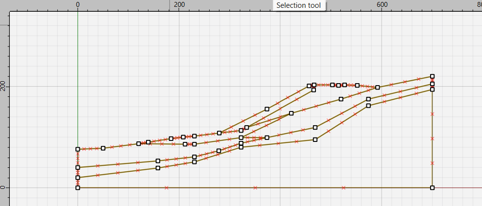
 ) on the
  ) to set zone length to 4. Then use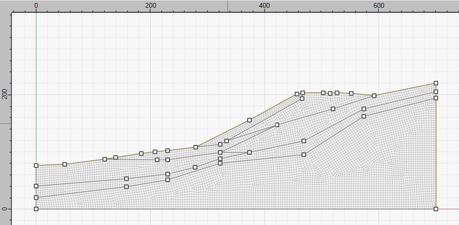
 ) to create the zones.
 from the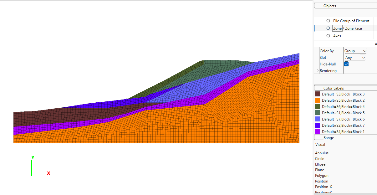
 ), and select the