Homogeneous Rock Slope with Benches (FLAC2D)

Example Application

This example reproduces Example 1.4.5 from the FLAC/Slope 8.1 manual. The project file for this example may be viewed/run in FLAC2D.[1] The main data file used is shown at the end of this example.

How To Read and Use Examples

Problem Statement

This example is a slope excavated in highly weathered granitic rock. The slope contains three 15 m high benches with two 8 m wide berms. The bench faces are inclined at 75 degress to the horizontal, and the top of the slope is cut at 45 degrees from the top of the third bench to the ground surface. Figure 1: illustrates the geometry of the slope. This example is taken from Wyllie and Mah (2004) which is based upon the example from Hoek and Bray (1981).

Figure 1: Failure surface solution from Bishop’s method for a rock slope (Wyllie and Mah 2004).

The rock mass is classified as a Hoek-Brown material. In the reference by Wyllie and Mah, 2004, the material properties are:

• GSI = 20

• mi = 15

• \(σ_{ci}\) = 150 MPa

• D = 0.7

For the Bishop’s method, a tangent to the curved Hoek-Brown failure envelope is drawn at a normal stress level estimated from the slope geometry. Equivalent Mohr-Coulomb properties for friction angle and cohesive strength are estimated by Wyllie and Mah (2004) to be

• φ = 43°

• c = 0.145 MPa

The mass density of the dry rock mass is 2500 kg/m3, and the mass density of the saturated rock mass is 2800 kg/m3. The phreatic surface is located as shown in Figure 1, and the mass density of water is 1000 kg/m3. Based upon these parameters, Wyllie and Mah report that the Bishop method produces a location for the circular failure surface and tension crack, as shown in Figure 1, and a factor of safety of 1.39.

You can explore possible best-fit Mohr-Coulomb envelopes using the Hoek-Brown rapid tool in FLAC2D. From the blue drop-down menu at the top of the workspace, select Rapid Tools - Hoek-Brown. You can enter the Hoek-Brown material properties above to see the Hoek-Brown curve. For the Mohr-Coulomb fit, under Failure Envelope Range, Select Slopes from the drop-down menu and enter a unit weight of 0.028 and a slope height of 20 m. You will see a calculated cohesion and friction angle similar to that used by Wyllie and Mah in their limit equilibrium analysis.

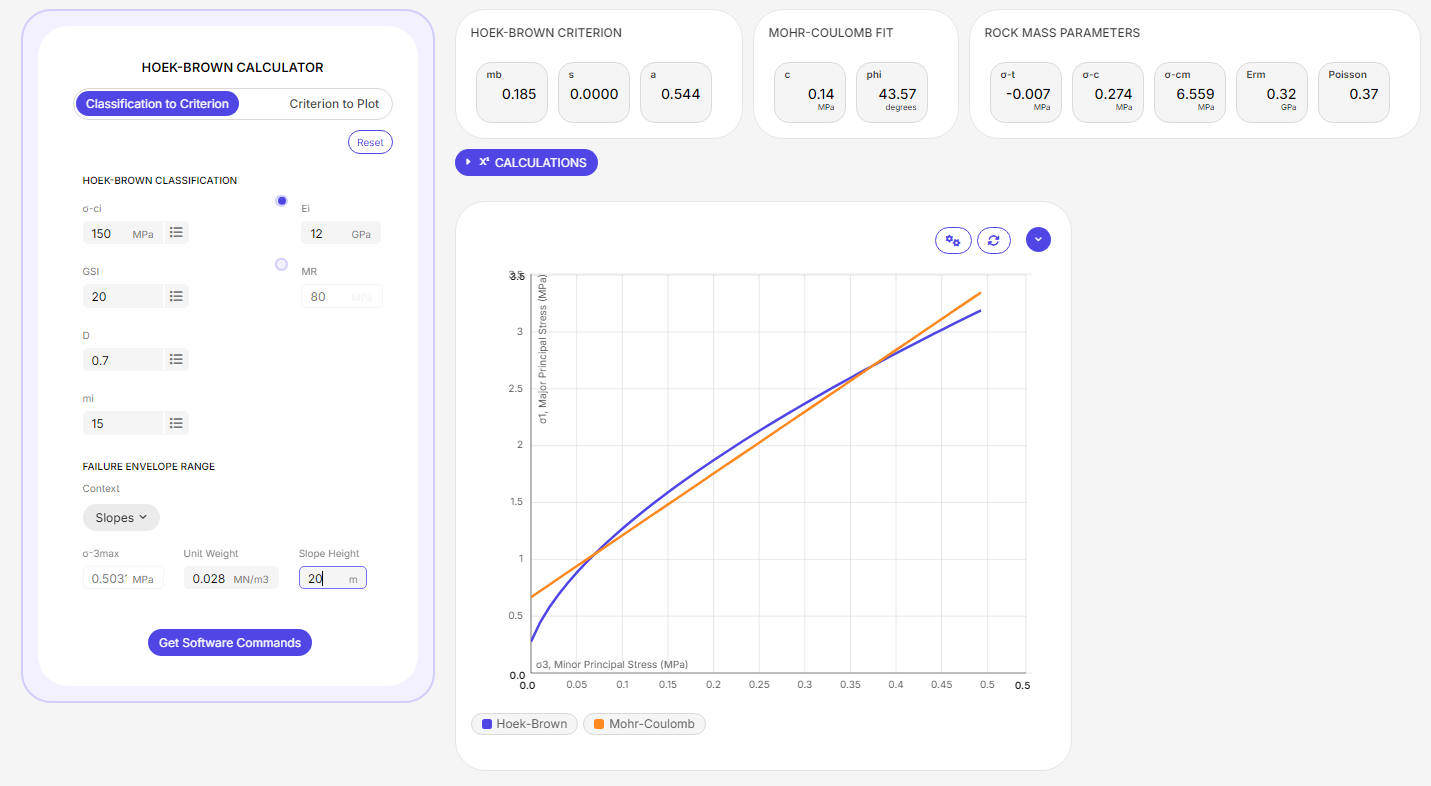
Figure 2: Hoek-brown failure envelope with best-fit Mohr-coulomb envelope

Model Setup

Model Geometry

The model zones are created in a sketch using the Slope Wizard tool. From the Slope Wizard tool, select bench-2 and enter the following parameters.

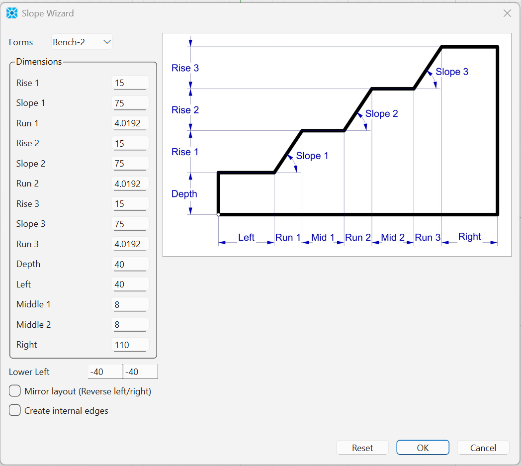
This creates a model with the benches. Note that you do not need to enter the run values. These are automatically calculated from the rise and the slope angle.

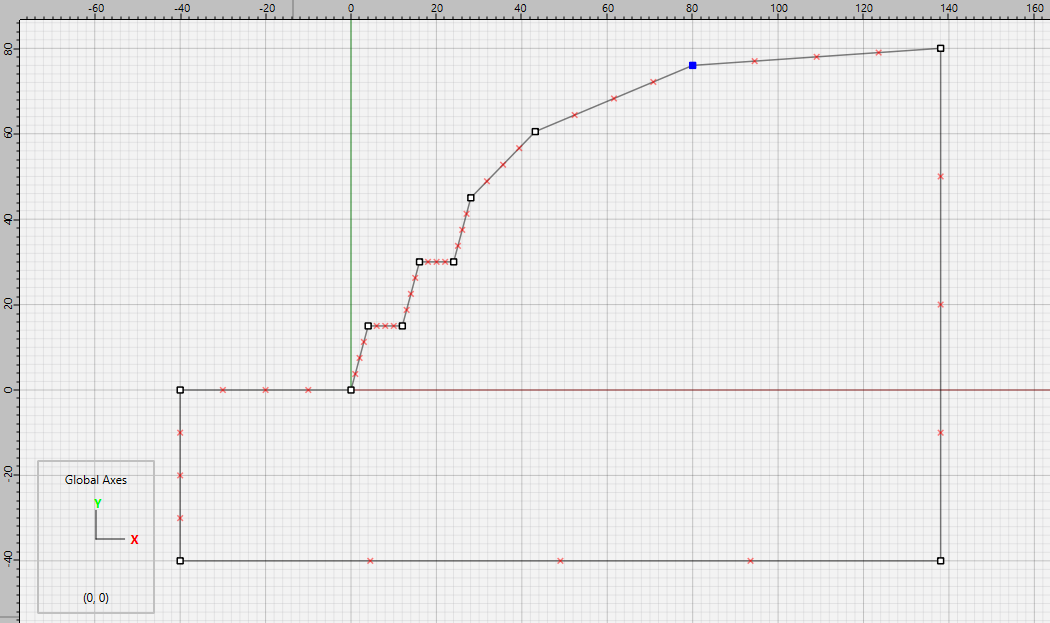
The top part of the slope now needs to be modified. Select the top-right point and change its y-coordinate to 80. Use the Point tool to add two new points to the top part of the slope. Click on the left-most new point and set its coordinates to (43.5,60.5) then click the other new point and set its coordinates to (80.5,76). The slope should now appear as shown.

Select Auto-size from the mesh drop-down menu and set the zone size to 2. Now select Mesh All Polygons . The final mesh is shown in Figure 5.

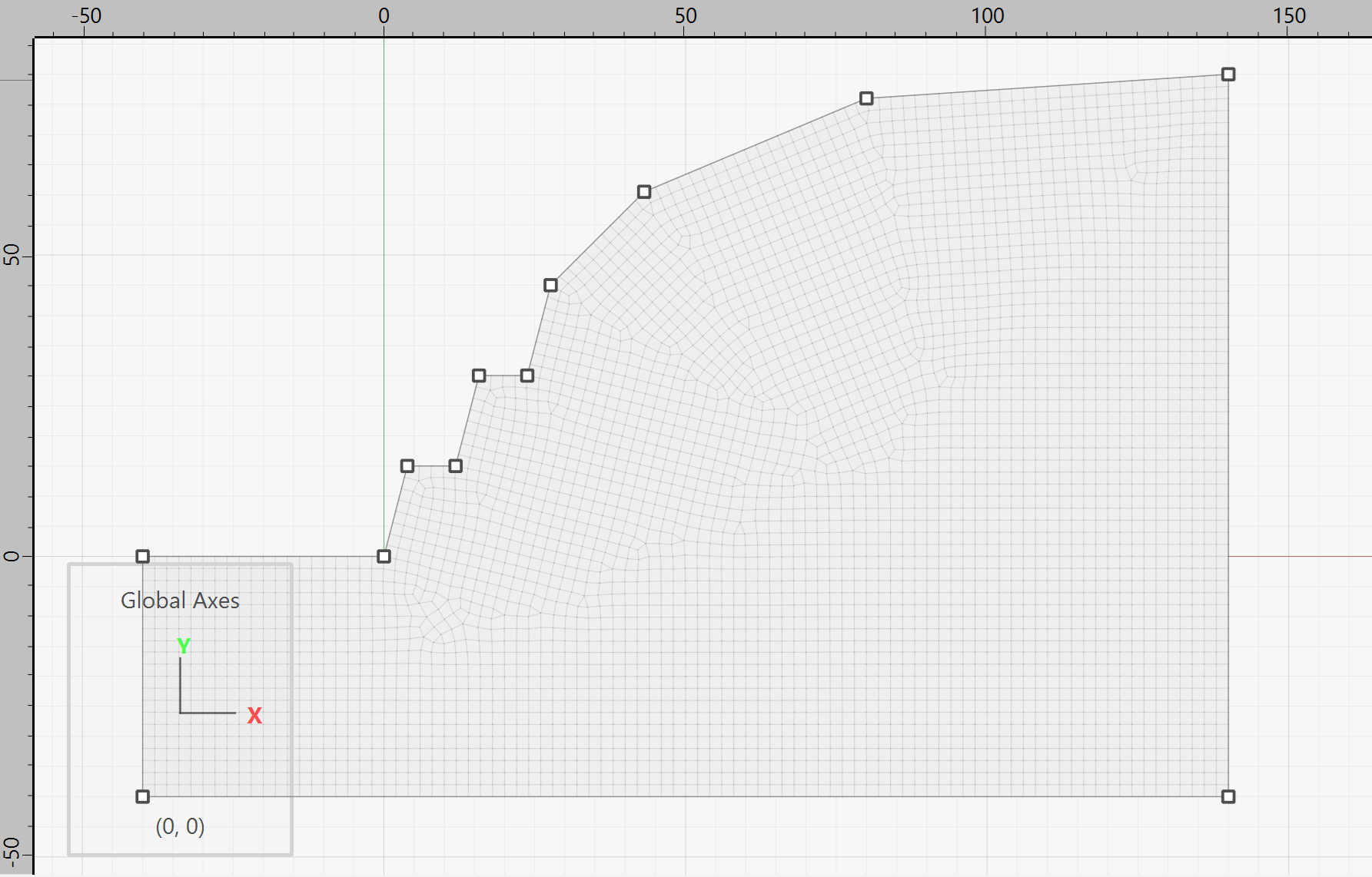
Figure 5: Rock bench mesh.

Click the button to Create Zones and save the project and the model state. Optionally, you can also select the State Record tab above the console pane, right click, and select Save to file as Data File.

Water Table

For the rest of the modeling, commands are used in a data file as shown in bench.dat. First, gravity is assigned and the Hoek-Brown properties are set. The model also contains a water table as shown in Figure 6. For a non-planar water table, the water table must first be defined as a geometry. This can be imported as a 2D dxf, or as a table of points. In this example, we will just create the geomtry wity commands as shown below. The geometry set is then specified when giving the zone gridpoint pore-pressure geometry command and pore-pressures will be automatically calculated.

geometry set 'water_table'
geometry edge create by-positions (-40.0,0.0) (0.0,0.0) (3.88,4.5) ...
            (11.88,12.0) (15.76,16.0) (23.76,24.0) (27.62,27.5) ...
            (43.15,39.5) (52.0,43.0) (80.0,48.0) (140.0,50.0)

; set water table. Pore pressures will be calculated
zone fluid-density = 1000
zone gridpoint pore-pressure geometry 'water_table' cutoff

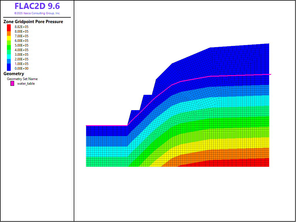
Figure 6: Water table and pore pressures for the rock slope.

Note that the wet density below the water table must also be supplied. Assuming a porosity of 0.3, the wet density can therefore be assigned as shown below.

[wet_dens = 2500 + 1000*0.3]

zone property density [wet_dens] ...
  range geometry-space 'water_table' count 1

Finally, the boundary conditions are applied by first giving the command zone face skin to automatically assign group names to the outer edges. These group names are then used as ranges when applying the boundary conditions.

Results

The model is run with a factor of safety calculation, The factor-of-safety is 1.32. The velocity vector plot (Figure 7) defines a failure region that closely resembles the failure surface produced from the Bishop solution.

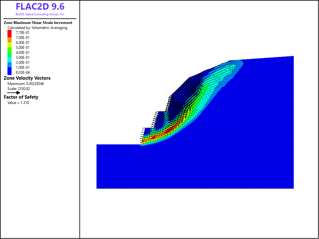
Figure 7: Shear strain contours and velocity vectors for the unstable state

References

Wyllie, D. C. and C. W. Mah. Rock Slope Engineering: Fourth Edition. Taylor and Francis Group (2004).

Data Files

bench.dat

model restore 'mesh'
model gravity 9.81
model large-strain off

zone cmodel assign hoek-brown

zone property density 2500.0 bulk 1E8 shear 3E7 ... 
              geological-strength-index 20 ...
              constant-mi 15 disturbance 0.7 ...
              constant-sci=1.5E8 tension=7480.0 ...
              flag-evolution=1

; make geometry set to define plane
geometry set 'water_table'
geometry edge create by-positions (-40.0,0.0) (0.0,0.0) (3.88,4.5) ...
            (11.88,12.0) (15.76,16.0) (23.76,24.0) (27.62,27.5) ...
            (43.15,39.5) (52.0,43.0) (80.0,48.0) (140.0,50.0)

; set water table. Pore pressures will be calculated
zone fluid-density = 1000
zone gridpoint pore-pressure geometry 'water_table' cutoff

; set wet density for zones below the water table
; assume a porosity of 0.3
[wet_dens = 2500 + 1000*0.3]

zone property density [wet_dens] ...
  range geometry-space 'water_table' count 1

zone face skin
zone face apply velocity-x 0 range group 'East' or 'West3'
zone face apply velocity (0,0) range group 'Bottom'

model factor-of-safety filename 'bench'

Endnote

[1]

This example is listed under the present document title in the i Examples dialog (use the menu command Help -> Examples… to access).