Oedometer Tests using CASM

Note

The project file for this example is available to be viewed/run in FLAC3D. The project’s main data files are shown at the end of this example.

The Clay-and-Sand model is used to simulate oedometer tests that vary the parameter of potential-exponent \(m\) and check its sensitivity to the ultimate stress ratio (horizontal to vertical) at rest \(K_0\).

The material properties are summarized in the table below.

critical-state-1	\(\Gamma\)	1.2
critical-state-2	\(\lambda\)	0.06
ratio-critical	\(M\)	1.2
pressure-reference	\(p_{ref}\)	100 (kPa)
kappa	\(\kappa\)	0.008
poisson	\(\nu\)	0.25
potential-exponent	\(m\)	1.5/2.0/2.5/3.0/3.5/4.0
yield-exponent	\(n\)	4.5
spacing-ratio	\(R\)	20
OCR-initial	\(OCR_0\)	1
stress-initial	\(\sigma_0\)	[tensor(-1,-1,-1,0,0,0)]

The results of stress ratio evolution due to compression in the oedometer tests are shown in Figure 1 to Figure 4. These results correctly reproduce the expected evolution path. Different values of \(m\) yield different \(K_0\) values, which match very well with the calibration equations between \(m\) and \(K_0\) provided in the CASM documentation. As \(m\) increases, the resulting \(K_0\) decreases.

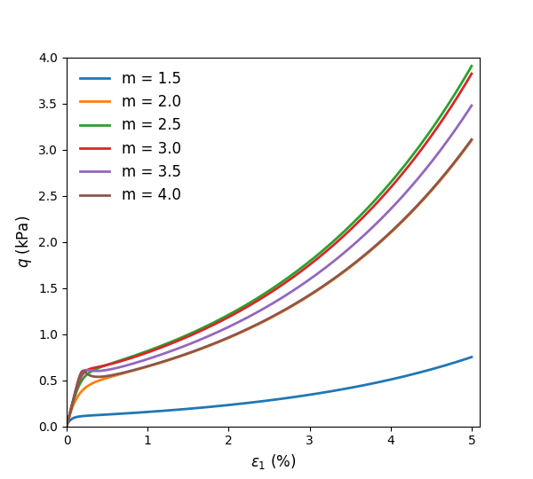
Figure 1: Simulated \(q\) vs. \(e_1\) of oedometer tests with varying \(m\).

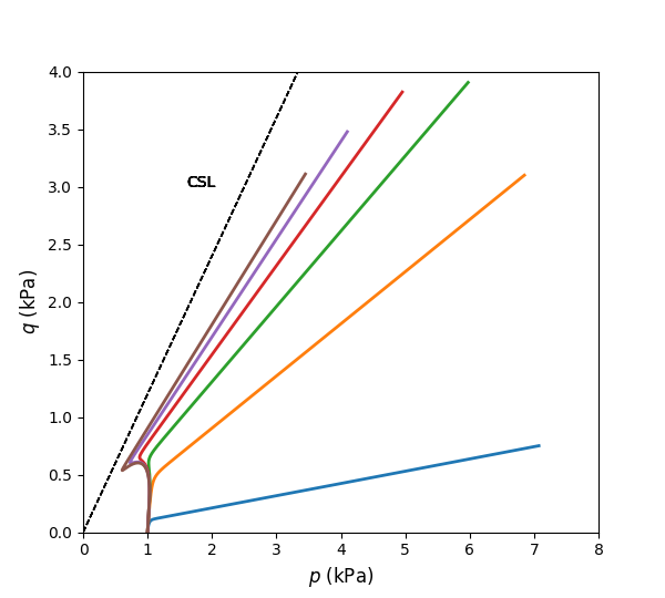
Figure 2: Simulated \(q\) vs. \(p\) of oedometer tests with varying \(m\).

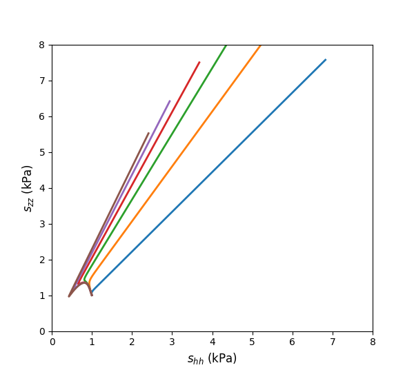
Figure 3: Simulated \(s_{hh}\) vs. \(s_{zz}\) of oedometer tests with varying \(m\).

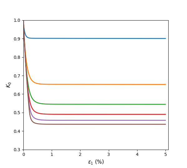
Figure 4: Simulated \(K_0\) vs. \(e_1\) of oedometer tests with varying \(m\).

Data Files

main-oedometer.py

import itasca as it
import numpy as np

paralist = [1.5, 2.0, 2.5, 3.0, 3.5, 4.0]

for m in paralist :
    outfile = 'oedometer_' + 'm_' + '{:3.2f}'.format(m)
    it.command("model new")
    it.fish.set('m', m)
    it.fish.set('savefile', outfile + '.f3sav')
    it.fish.set('txtfile',  outfile + '.txt')
    it.command("program call 'oedometer.dat' ")
    
    

oedometer.dat

;model new
; Oedometer Test
model large-strain off
zone create brick size 1 1 1
zone cmodel assign clay-and-sand
; 
zone property critical-state-1 1.2
zone property critical-state-2 0.06
zone property pressure-reference 100.0
zone property kappa 0.008
zone property ratio-critical 1.2
zone property yield-exponent 4.5
zone property potential-exponent [m]
zone property spacing-ratio 20
zone property poisson 0.25
zone property ocr-initial 1.0
;
zone initialize stress xx -1.0 yy -1.0 zz -1.0
;
zone property stress-initial [tensor(-1,-1,-1,0,0,0)]
;
zone gridpoint fix velocity
zone face apply velocity-z -1e-6 range position-z 1
;
[global zn = zone.near(0.5, 0.5, 0.5)]
[global gp = gp.near(1.0,1.0,1.0)]
fish define e1
    global e1 = -gp.disp.z(gp)*100.
    local stress = zone.stress(zn)
    global sxx = -stress->xx 
    global syy = -stress->yy 
    global szz = -stress->zz
    global shh = 0.5*(sxx + syy)
    global q = szz - shh
    global p = (sxx + syy + szz)/(3)
    global k0 = shh / szz    
end
zone history displacement-z position 0 0 1
zone history stress-zz position 0.5 0.5 0.5
fish history name 'e1' e1
fish history name 'shh' shh
fish history name 'szz' szz
fish history name 'p'  p
fish history name 'q'  q
fish history name 'k0' k0
history interval 10

model solve-static cycles 50000

history export 'e1', 'shh', 'szz', 'p', 'q', 'k0' file [txtfile] truncate
model save [savefile]