FLAC3D Theory and Background • Constitutive Models

Clay-and-Sand Model (CASM)*

Note

*Not available in 3DEC.

The Clay-and-Sand Model (CASM) is a unified critical state constitutive model applicable to both clay and sand. It was initially proposed by Yu (1998) and later slightly modified by Arroyo and Gens (2021). CASM extends the original and modified Cam-Clay models by incorporating an exponent in the yield function, allowing it to represent a general stress state associated with the reference consolidation line. This enhancement enables CASM to overcome key limitations of the Cam-Clay model, which is valid only for normally consolidated or slightly over-consolidated clays.

Key features of CASM include:

• The ability to reproduce strain-softening behavior in over-consolidated clays and dense sands, as well as strain-hardening responses in normally consolidated clays and loose sands.

• A relatively small set of material parameters, most of which can be calibrated from standard laboratory tests such as triaxial compression and oedometer tests.

• The capability to capture and control both peak and residual undrained strengths under undrained triaxial loading, as well as the ultimate stress ratio in one-dimensional consolidation conditions.

• Suitability for the assessment of static liquefaction potential.

Formulations

Unless explicitly stated otherwise, all stresses are expressed in terms of effective stress. The Itasca stress sign convention is adopted: tensile stresses are considered positive, while compressive stresses are negative. An exception is made for mean effective stress and pore pressure, both of which are taken as positive in compression. Principal stresses are ordered such that \(\sigma_1 \le \sigma_2 \le \sigma_3\).

Critical State and Reference State

As shown in Figure 1, the critical state line (CSL) is assumed to represent a strength line in the plane of void ratio (\(e\)) versus the logarithm of mean effective pressure (\(\ln{p}\)):

(1)\[ e_c(p) = \Gamma - \lambda \ln{\left( \frac{100p}{p_{ref}} \right)}\]

where \(\Gamma\) and \(\lambda\) are material constants. Here \(100/p_{ref}\) is used for unit normalization so that when \({p_{ref}}\) is taken the typical value of 100 kPa, \(\Gamma\) is the critical-state void ratio at 1 kPa.

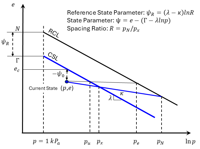
Figure 1: Schematics of state-parameter, critical state constants and reference state parameter if stress is in kPa.

The state parameter is defined as the difference between the current void ratio and the critical-state void ratio at the same mean effective pressure:

(2)\[ \psi = e - e_c(p)\]

A reference consolidation line (RCL) is assumed parallel to CSL:

(3)\[ e_N(p) = N - \lambda \ln{\left( \frac{100p}{p_{ref}} \right)}\]

where \(N\) is the reference consolidation void ratio at 1 kPa.

For clays, the isotropic Normal Consolidation Line (NCL) is typically used as the RCL. However, for some sands, the NCL may not be accurately measurable. In such cases, the reference state parameter can be selected to correspond to a condition that the soil is unlikely to reach in practice (Yu, 1998).

The distance between \(N\) and \(\Gamma\) is the critical-state void ratio at 1 kPa is defined as the reference state parameter denoted by \(\psi_R = N - \Gamma\). In the original Cam-Clay (OCC) model, \(\psi_R = \lambda - \kappa\), where \(\lambda\) and \(\kappa\) are the slopes of CSL and the swelling line, respectively, as shown in Figure 1, while in the modified Cam-Caly (MCC) model, \(\psi_R = (\lambda - \kappa)\ln{2}\).

In CASM, a general formulation is assumed

(4)\[\psi_R = (\lambda - \kappa) \ln {R}\]

where \(R\) is a material constant referred to as the spacing ratio, defined as the ratio of the pressure at NCL (\(p_N\)) and the pressure at CSL (\(p_x\)) if along the swelling line passing through the current state \((p,e)\) (see Figure 1):

(5)\[R = p_N / p_x\]

Apparently, the OCC model corresponds to the special case where \(R=\exp(1)\) , and the MCC model corresponds to \(R=2\).

Elastic Law

Similar to the Cam-Clay model, CASM employs an isotropic nonlinear elastic formulation, based on the assumption of a straight elastic unloading–reloading (swelling) line in the \(e\) vs. \(\ln{p}\) space. The elastic bulk modulus is expressed as:

(6)\[K = \frac{(1+e)p}{\kappa}\]

where \(\kappa\) is the slope of the swelling line in the plane of \(e-\ln{p}\) (see Figure 1).

The elastic shear modulus is then computed from the current bulk modulus and a constant Poisson’s ratio (\(\nu\)), assumed to be a material property:

(7)\[G = \frac{3(1-2\nu)}{2(1+\nu)} K\]

Yield Function

CASM assumes a yield function

(8)\[f = \left( \frac{q}{M_{\theta}p} \right)^n + \frac{1}{\ln{R}} \ln{\left( \frac{p}{p_N} \right)}\]

where \(n\) is a material constant that controls slope of shape of the yield function; \(q = \sqrt{(3s_{ij}s_{ij})/2}\) and \(s_{ij}\) is the deviatoric stress tensor, \(p = -\sigma_{ii}/3\) is the mean effective stress; \(M_{\theta}\) is the slope of the CSL in the q vs. p plane that depends on the Lode’s angle \(\theta\):

(9)\[ \theta = {{1} \over {3}} \arcsin{\left( -{{27} \over {2}} {{J_3} \over {q^3}} \right)}\]

where \(J_3 = (s_{ij}s_{jk}s_{ki})/3\). The Lode’s angle is in the range of \([-\pi/6, \pi/6]\) by the aforementioned definition and for triaxial compression condition, \(\theta = \pi/6\) and for triaxial extension condition, \(\theta = -\pi/6\).

(10)\[ M_{\theta} = r(\theta) M\]

where \(M\) is a material constant representing \(\eta = q/p\) at the critical state in the TC (triaxial compression) condition, \(r(\theta)\) is a function considering the effect of the Lode’s angle \(\theta\), defined by

(11)\[r(\theta) = \left( \frac{1+c^{-4}}{2} + \frac{1-c^{-4}}{2} \sin{3\theta} \right)^{-0.25}\]

to interpolate \(M_{\theta}\) for a given Lode angle \(\theta\) and the strength ratio \(c\), which is defined by \(c = 3/(3+M)\). For triaxial compression condition (\(\theta = \pi/6\)), \(r=1\) and \(\partial r/\partial \theta = 0\); for triaxial extension condition (\(\theta = -\pi/6\)), \(r=c\), and \(\partial r/\partial \theta = 0\).

The normalized yield surfaces by varying \(n\) and \(R\) values are shown in Figure 2 and Figure 3, respectively.

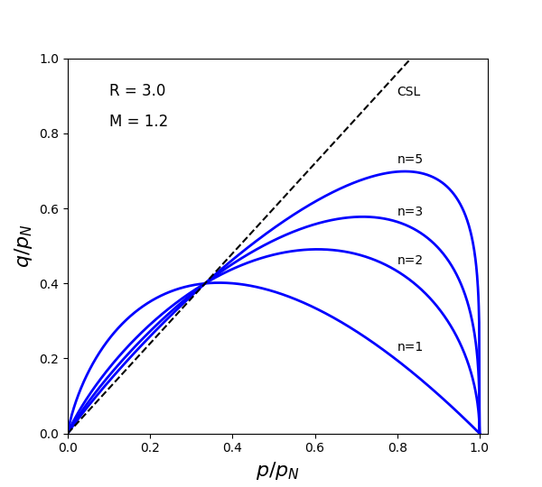
Figure 2: Normalized yield surfaces with various \(n\).

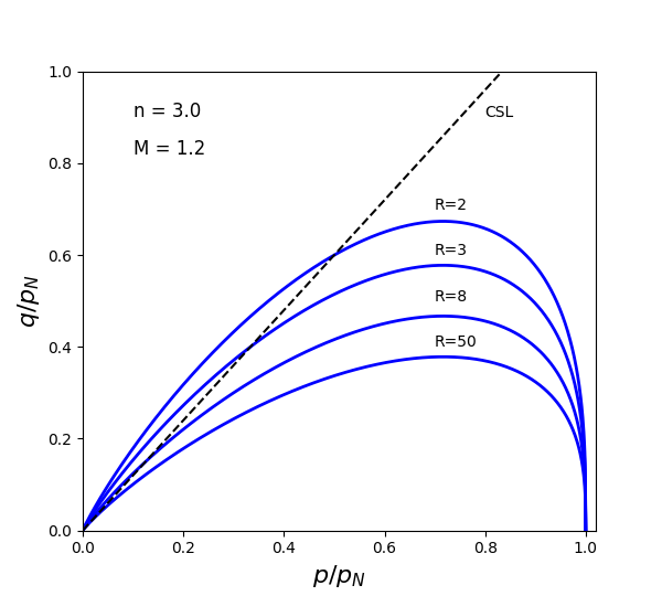
Figure 3: Normalized yield surfaces with various \(R\).

CASM yield function can be alternatively given by

(12)\[f = \left( \frac{\eta}{M_{\theta}} \right)^n + \frac{\psi}{\psi_R} - 1\]

If neglecting Lode’s angle effect, the OCC model is recovered by \(\psi_R = \lambda - \kappa\) and \(n=1\), and the MCC model can be approximated by setting \(\psi_R = (\lambda - \kappa) \ln{2}\) and a suitable \(n\) value (Yu, 1998). The stress-state relations for OCC, MCC and CASM are plotted in Figure 4.

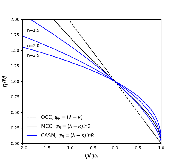
Figure 4: Stress-state relations for original and modified Cam-Clay, and CASM with varying \(n\).

Plastic Potential Function

The original CASM plastic potential function (Yu 1998) was defined as

(13)\[g = 3M_{\theta} \ln{(p/\beta)} + (3+2M_{\theta})\ln{( 3+2\eta)} - (3-M_{\theta})\ln{( 3-\eta)}\]

where the size parameter \(\beta\) can be determined for any given stress state \((p,q, \theta)\) by solving \(g = 0\). This plastic potential function is non-associated as it differs from the yield function.

Arroyo and Gens (2021) proposed an alternative non-associated plastic potential function, given by

(14)\[g = \left( \frac{q}{M_{\theta}p} \right)^m + (m - 1) \left( 1 - \frac{p_M}{p} \right)\]

where \(p_M\) must be obtained based on the given stress state \((p,q, \theta)\) by solving \(g=0\) and \(m\) (limited to \(m > 1\)) is a material constant which allows adjusting the desired stress ratio for 1D consolidation. The normalized potential surfaces with various \(m\) are shown in Figure 5.

To incorporate both forms of the plastic potential function defined by Equations (13) and (14), the following rule is applied: if \(m = -1\), Equation (13) is used, and if \(m > 1\), Equation (14) is used. Other values assigned to \(m\) are not allowed.

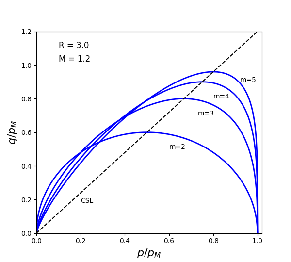
Figure 5: Normalized potential surfaces with various \(m\).

Plastic Hardening Rule

CASM uses the same isotropic volumetric plastic strain hardening rule as the MCC model:

(15)\[\dot{p}_N = - \frac{(1+e)p_N}{\lambda - \kappa} \dot{\epsilon}^p_{v}\]

where \(\epsilon^p_{v}\) is the volumetric plastic strain.

Model Properties

Property Calibration

The mandatory model properties (material constants) for the CASM model are:

• \(p_{ref}\) — the reference pressure used for stress normalization. This is typically set to 100.0 when using kPa as the stress unit, or its equivalent in other units.

• \(\Gamma\), \(\lambda\), and \(M\) — the critical state parameters. Estimating these constants is relatively straightforward for clay soils, but more challenging for sands. Special care must be taken when determining these values using triaxial tests.

  • The parameter \(\Gamma\) which is the void ratio at the critical state line when \(p\) = 1 kPa. generally falls within the range of 0.8 to 3.0 for various soils.

  • Typical values of \(\lambda\) range from 0.01 to 0.05 for sands at relatively low confining pressures (e.g., less than 1000 kPa). However, in high-pressure regimes, larger values may be observed. For clays, \(\lambda\) typically ranges from 0.1 to 0.2.

  • The parameter \(M\) is the ratio of \(q/p\) (or \(\eta\)) at the critical state corresponding to triaxial compression state. It can be determined from drained or undrained triaxial tests with pore pressure measurements on isotropically consolidated samples. To accurately assess \(M\), testing should proceed to sufficiently large strains to ensure that the soil approaches the critical state. Typical values of \(M\) range from 0.8 to 1.0 for clays and from 1.1 to 1.4 for sands.

• \(\kappa\) and \(\nu\) — parameters defining the elastic behavior.

  • The parameter \(\kappa\) is the slope of swelling line in the plane of \(e-\ln{p}\). For sands, a typical value of \(\kappa\) is approximately 0.005. For clays, \(\kappa\) is generally higher, commonly ranging from 0.01 to 0.06.

  • Poisson’s ratio \(\nu\) typically lies between 0.15 and 0.35 for both clays and sands.

• \(m\) is to define the plastic potential function.

The parameter \(m\) controls the plastic flow ratio and can be estimated from the coefficient of earth pressure at rest, \(K_0\). Based on the conditions of an oedometer test, a relationship between \(m\) and \(K_0\) can be established (Mánica et al., 2021):

(16)\[\frac{9(\lambda-\kappa)(2\nu-1)}{2\kappa(\nu+1)\eta_{K0} + 6\lambda(2\nu-1)} = \frac{1-m}{m} \left( \eta_{K0} - M^m {\eta_{K0}^{1-m}} \right)\]

where \(\eta_{K0} = 3(1-K_0)/(1+2K_0)\).

If neglecting relatively small part from elastic strain since \(kappa\) is relatively small, a simplified approximate version of Equation (16) can be:

(17)\[\frac{3}{2} \Lambda = \frac{1-m}{m} \left( \eta_{K0} - M^m {\eta_{K0}^{1-m}}\right)\]

where \(\Lambda = (\lambda-\kappa)/\lambda\).

For a target coefficient of earth pressure at rest, \(K_0\), the parameter \(m\) can be solved from the implicit relation between \(m\) and \(K_0\) (via \(\eta_{K0}\)) in Equation (16) or (17) using an iteration method, provided that other parameters (\(M\), \(\lambda\), \(\kappa\) and \(\nu\)) are known. Figure 6 compares the analytical solutions of Equation (16) and (17) with the back-calculated \(m\) values based on the FLAC3D numerical Oedometer Tests, showing good agreement. An increase in \(K_0\) is associated with a decrease in \(m\).

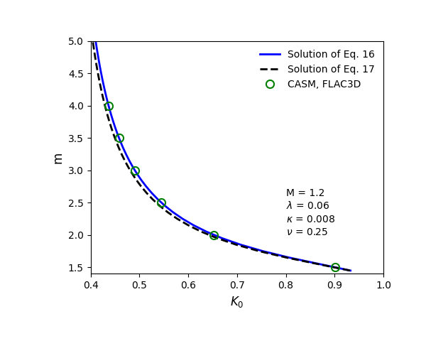
Figure 6: Analytical solutions and back-calculated \(m\).

• \(R\) and \(n\) to define the shape of yield surface.

The spacing ratio \(R\) is used to estimate the reference state parameter, which corresponds to the loosest state a soil is likely to reach in practice.While this assumption is reasonable for clays, it has proven less suitable for sands. Experimental data suggest that for clays, \(R\) typically falls within the range of 1.5 to 3.0, whereas for sands, it is generally much higher. In most applications, it is sufficient to treat the normal consolidation line (NCL) as the reference consolidation line (RCL). As the NCL is readily identifiable for clays, measuring \(R\) poses no significant challenge. However, identifying NCL for sands is more difficult, as it requires a testing device capable of applying very high pressures. When direct measurement of NCL is not feasible, it is acceptable to define \(R\) so that the reference state (\(\xi_R\)) using a positive state parameter, typically in the range of 0.05 to 0.2, that is unlikely to be encountered in practice.

The parameter \(R\) can be calibrated from the residual (critical state) undrained strength \(S_{ur}\). Take the isotropically consolidated undrained triaxial test as an example:

(18)\[R = OCR_0 \left( \frac{M}{2} \frac{p_0}{S_{ur}} \right)^{1 \over \Lambda}\]

where \(p_0\) is the initial isotropically consolidated stress and \(OCR_0\) is the initial over-consolidation ratio. For natural deposits,

(19)\[R = OCR_0 \left[ \frac{M (1+2K_0)}{6} \left( \frac{\sigma'_{v0}}{S_{ur}} \right) \right]^{1 \over \Lambda}\]

where \(\sigma'_{v0}\) is the deposit effective vertical stress and \(K_0\) is the coefficient of earth pressure at rest. \({S_{ur}}/{\sigma'_{v0}}\) can be directly correlated from the cone tip resistance.

The parameter \(n\) can be calibrated (Cirone et al 2025) from the slope of the instability line denoted by the stress ratio, \(\eta_{IL}\), defined at the state with the maximum \(q\) during an undrained triaxial compression test:

(20)\[\eta_{IL} = \frac{M}{\sqrt[n]{n\ln{R}}} = M \left( n \frac{\psi_R}{\lambda} \right)^{-1/n}\]

the parameter \(n\) can thus be solved based on the value of \(\eta_{IL}\) and other known parameters from Equation (20).

Properties for Initial Conditions

CASM is a stress-dependent model, so the initial stress tensor must be specified to calculate the initial elastic moduli when the model is first assigned. In addition to the mandatory initial stress tensor, \(\boldsymbol{\sigma}_0\), at least one of the following initial parameters must also be provided : the initial void ratio (\(e_0\)), the initial state parameter (\(\psi_0\)), or the initial over-consolidation ratio (\(OCR_0\)). In all cases, the input or calculated \(\psi_0\) should meet \(\psi_0 \le (\lambda - \kappa) ln{R}\).

• Using initial void ratio, \(e_0\):

The other parameters are internally initialized by

(21)\[\psi_0 = \Gamma - \lambda \ln{\left( \frac{100 p_0}{p_{ref}} \right)} - e_0\]

(22)\[p_N = R \exp{\left[ \frac{\Gamma - \kappa \ln{\left( \frac{100 p_0}{p_{ref}} \right)} - e_0 }{\lambda - \kappa} \right]}\]

(23)\[OCR_0 = \frac{p_N}{\exp{\left[ \left( \frac{q}{M_{\theta} p} \right)^n_0 \ln{R} \right]}}\]

• Using initial state parameter, \(\psi_0\):

The other parameters are internally initialized by

(24)\[e_0 = \Gamma - \lambda \ln{\left( \frac{100 p_0}{p_{ref}} \right)} + \psi_0\]

Other calculations are the same as Equations (22) and (23).

• Using initial OCR, \(OCR_0\):

The other parameters are internally initialized by

(25)\[p_N = {p_0} \times {\exp{\left[ \left( \frac{q}{M_{\theta} p} \right)^n_0 \ln{R} \right]}} \times OCR_0\]

(26)\[p_x = p_N / R\]

(27)\[e_0 = \Gamma - (\lambda - \kappa) \ln{{p_x}} - \kappa \ln{\left( \frac{100 p_0}{p_{ref}} \right)}\]

(28)\[\psi_0 = e_0 - \Gamma + \lambda \ln{\left( \frac{100 p_0}{p_{ref}} \right)}\]

Property List

Table 1: Sand-and-Clay Model material property names

Category	Names	Note
Unit Normalization	pressure-reference (\(p_{ref}\))	100 kPa
Elasticity	kappa (\(\kappa\))
	poisson (\(\nu\))	default 0.2
Critical State	critical-state-1 (\(\Gamma\))
	critical-state-2 (\(\lambda\))
	ratio-critical (\(M\))
Yield Function	yield-exponent (\(n\))	\(n \ge 1\)
	spacing-ratio (\(R\))	\(R > 1\)
Potential Function	potential-exponent (\(m\))	\(m\) > 1 or \(m\) = -1
Initial Condition	stress-initial (\(\sigma_0\))	tensor
	void-initial (\(e_0\)), or
	state-parameter-initial (\(\xi_0\)), or	\(\xi_0 \le \xi_R\)
	OCR-initial (\(OCR_0\))	\(OCR_0 \ge 1\)
Read-Only	bulk (\(K\))
	shear (\(G\))
	void (\(e\))
	state-parameter (\(\xi\))
	pressure-cap (\(p_N\))
	pressure-effective (\(p\))

References

Arroyo, M. and Gens, A. Computational analyses of Dam I failure at the Corrego de Feijao mine in Brumadinho. Final Report for VALE SA. (2021).

Cirone, N.M, Rasmussen, R.E., & Delgado, B. CASM model: strength, instability line, and brittleness index in undrained triaxial compression. Canadian Geotechnical Journal, 62, (2025).

Mánica, M. A., Arroyo, M., Gens, A., & Monforte, L. Application of a critical state model to the Merriespruit tailings dam failure. Proceedings of the Institution of Civil Engineers-Geotechnical Engineering, 175(2), 151-165 (2021).

Yu, H.S. CASM: a unified state parameter model for clay and sand. International Journal for Numerical and Analytical Methods in Geomechanics, 22(8), 612-753 (1998).

Examples

Drained and Undrained Triaxial Tests of Weald Clay
Drained Triaxial Tests of Erksak Sand
Undrained Triaxial Tests of Loose Ottawa Sand
Oedometer Tests
Tailing Dam Static Liquefaction (FLAC3D)
Tailing Dam Static Liquefaction (FLAC2D)

clay-and-sand Model Properties

Use the following keywords with the zone property command to set these properties of the Clay and Sand model (CASM).

clay-and-sand

critical-state-1 f

critical state parameters, \(\Gamma\). This value represents the void ratio (not the specific volume, as used in some literature) at the critical state when \(p\) = 1 kPa. is the Typical values are in 0.8 to 3.0.

critical-state-2 f

critical state parameters, or slope of normal consolidation line, \(\lambda\). It should be greater than \(\kappa\). Typical value are 0.01 to 0.05 for sands, and 0.1 to 0.2 for clays.

kappa f

slope of elastic swelling line, \(\kappa\). It should be less than \(\lambda\). Typical values is around 0.005 for sands and 0.01 to 0.06 for clays.

pressure-reference f

reference pressure, \(p_{ref}\). The value takes usually 100.0 if in kPa, or the equivalent in other units.

ratio-critical f

stress ratio \(q/p\) at critical state in the triaxial compression test, \(M\). Typical value is 0.8 to 1.0 for clays and 1.1 to 1.4 fro sands.

spacing-ratio f

spacing ratio, \(R\). Typical values are 1.5 to 3.0 fro clays and much larger (to thousands) for sands.

potential-exponent f

exponent in the plastic potential function, \(m\). Typical values are 2.0 to 4.0. If \(m = -1\), the original Yu (1998) plastic potential function is used.

yield-exponent f

exponent in the yield function, \(n\). Typical values are 1.0 to 5.0.

poisson f (a)

Poisson’s ratio, \(\nu\). Typical values are 0.15 to 0.35 for sands and clays. The default value is 0.2.

ocr-initial f (i)

initial over consolidation ratio, \(OCR_0\). Allowable values are 1.0 or more.

state-parameter-initial f (i)

initial state parameter, \(\psi_0\). Allowable maximum value is \((\lambda - \kappa) \ln{R}\).

stress-initial :tensor:`t` (i)

initial stress tensor, \(\sigma_{ij,0}\). It should not be outside of the initial yield surface.

void-initial f (i)

initial void ratio, \(e_0\).

bulk f (r)

current elastic bulk modulus, \(K\).

pressure-cap f (r)

current cap pressure of the yield surface, \(p_N\).

pressure-effective f (r)

current mean effective stress, \(p\).

shear f (r)

current elastic shear modulus, \(G\).

state-parameter f (r)

current state parameter, \(\psi\).

void f (r)

current void ratio, \(e\).

Key

(a) Advanced property.

This property has a default value; simpler applications of the model do not need to provide a value for it.

(i) Initial property.

This property will not be updated once initialized (first input).

(r) Read-only property.

This property cannot be set by the user. Instead, it can be listed, plotted, or accessed through FISH.