Saturation and Drainage of a Caisson (FLAC2D)

Problem Statement

Note

This project reproduces Example 2.5.1 from FLAC 8.1. The project file for this example is available to be viewed/run in FLAC2D.[1]. The project’s main data files are shown at the end of this example.

This one-dimensional example involves simulation of infiltration in a large caisson, and drainage by gravity following complete saturation. The geometry, properties, initial, and boundary conditions correspond to those of the Test Problem 1 in Forsyth and Wu (1995). The caisson is 6 m in height and 0.3 m in width. The water saturation is initially \(S_w\) = 0.303 throughout the caisson. Infiltration takes place at the rate of 0.2 m/day at the top of the caisson until it is fully saturated. Subsequently, drainage by gravity is allowed to take place at the bottom of the caisson for a period of 100 days. The material properties used in the model are those of the Bandelier Tuff (see Table 1 in Forsyth and Wu (1995)). These are listed in Table 1.

Table 1: Fluid properties

Property	Value
Porosity	0.33
Sat. mobility coefficient	2.92 \(\times\) 10-10 m2/Pa s
Intrinsic permeability	2.95 \(\times\) 10-13 m2
Wetting-phase viscosity	1.01 cP
Wetting-phase compressibility	0.001 kPa-1
Rock compressibility	0.0 kPa-1 (rigid)
Residual saturation	0.0
van Genuchten \(m\)	0.336
van Genuchten \(n\)	1.506
van Genuchten \(p_{ref}\)	7 kPa
Rel. permeability exponent \(b\)	0.5

A column of 20 zones is used to represent the caisson. During the infiltration phase, the bottom boundary is closed until fully saturated. After that, the wetting-phase pressure is kept constant at zero along the bottom boundary. Rock compressibility is assumed to be zero, i.e., rigid. Moreover, the relative permeability of the wetting-phase is given by:

(1)\[k_{rw} = S_{w}^{b} \left[ 1 - \left( 1 - S_{w}^{1/m}\right)^{m} \right]^{2}\]

where \(k_{rw}\) is the relative permeability of the wetting-phase, \(S_{w}\) is the water saturation, \(b\) is the relative permeability exponent, and \(m\) is a van Genuchten fitting parameter.

Changes in wetting-phase pressure \(p_w\) are governed by the following equation, assuming an isothermal, rigid skeleton:

(2)\[\frac{1}{M} \Delta p_w = \frac{1}{S_w} \Delta \zeta - \frac{\phi}{S_w} \Delta S_w \quad \mathrm{or, equivalently}\]

(3)\[\left(\frac{1}{M} - \frac{\phi}{S_w} \frac{\Delta S_w}{\Delta p_c}\right) \Delta p_w = \frac{1}{S_w} \Delta \zeta\]

where \(M\) is the saturated Biot modulus, \(\zeta\) is the variation of fluid content, \(\phi\) is the porosity, and \(p_c=-p_w\) is the capillary pressure, or suction. The term on the left hand side of equation (3) and in brackets is the inverse of the Biot modulus in partially saturated conditions. This value is stored as a FISH extra gridpoint variable during the drainage phase to visualize the impact of saturation on the Biot modulus.

Results

Figure 1 shows the water content profile (porosity times water saturation) over the caisson height at 1.16, 4.16, and 7.16 days. After complete saturation, the infiltration rate is set to zero and gravity drainage is simulated for 100 days. The predicted water content profile at 1, 4, 20, and 100 days is given in Figure 2. Lastly, the impact of saturation on the Biot modulus is shown in Figure 3. The Biot modulus is only equal to the value under fully saturated conditions at the bottom of the caisson (\(y=0\) m) where saturation is 1. Everywhere else in the caisson, partially saturated conditions prevail during drainage and this has a non-negligable impact on the transient response.

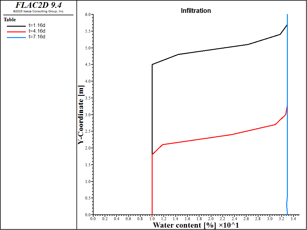
Figure 1: Water content profile during infiltration.

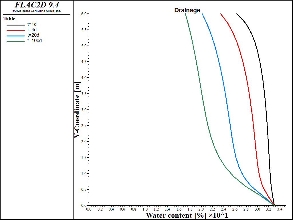
Figure 2: Water content profile during drainage.

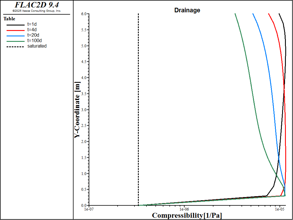
Figure 3: Compressibility profile during drainage. This is the inverse of the partially saturated Biot modulus.

Reference

Forsyth, P. A. and Y. S. Wu. “Robust numerical methods for saturated-unsaturated flow with dry initial conditions in heterogeneous media,” Advances in Water Resources, 18, 25-38 (1995).

Data Files

saturation_drainage.dat

model large-strain off
model configure fluid-flow
model gravity 0 -10

[Cw = 1e-6]   ; Wetting phase compressibility [1/Pa]
[Cnw = 1e-3]  ; Non-wetting phase compressibility [1/Pa]

[n = 1.506]   ; Van-Genuchten n
[m = 0.336]   ; Van-Genuchten m
[pr = 7e3]    ; Van-Genuchten pref [Pa]
[b = 0.5]     ; Relative permeability exponent

[q = 0.2 / 86400.0]  ; Wetting phase injection rate [m/s]

program call "functions"

zone create quadrilateral size 1 20 ...
    point 0 (0,0) point 1 (0.3,0) ...
    point 2(0,6)
    
zone fluid property fluid-density 1000 porosity 0.33 ...
    mobility-coefficient 2.92e-10 fluid-modulus [1/Cw]
zone fluid unsaturated van-genuchten [n] [m] [pr]

[init_pp]
[rel_perm]

zone fluid property effective-cutoff -1e20
zone fluid permeability-saturation table "krw"
zone face apply discharge [q] range position-y 6

fish callback add water_content -1 interval 10

; Step 1: Solve to fully-saturated
model solve-fluid time-total 1.0e5
[save_profile("wc_1.16d", 1)]
model solve-fluid time-total 3.6e5
[save_profile("wc_4.16d", 1)]
model solve-fluid time-total 6.2e5 fish-halt is_saturated
[save_profile("wc_7.16d", 1)]

; Remove injection, allow drainage
zone face apply-remove discharge range position-y 6
zone face apply pore-pressure 0 range position-y 0
model fluid time-total 0

fish callback add apparent_Cw -1 interval 10

; Solve for 100 days
model solve-fluid time-total [86400 * 1]
[save_profile("wc_1d", 1)]
[save_profile("ac_1d", 2)]
model solve-fluid time-total [86400 * 4]
[save_profile("wc_4d", 1)]
[save_profile("ac_4d", 2)]
model solve-fluid time-total [86400 * 20]
[save_profile("wc_20d", 1)]
[save_profile("ac_20d", 2)]
model solve-fluid time-total [86400 * 100]
[save_profile("wc_100d", 1)]
[save_profile("ac_100d", 2)]

functions.dat

fish define init_pp
    ; Initialize constant initial pore pressure
    local Swi = 0.303
    local pi = -pr * (Swi^(-1.0/m)- 1.0)^(1.0 - m)
    gp.pp(::gp.list) = pi
    gp.sat(::gp.list) = Swi
end

fish define rel_perm
    ; Wetting phase relative permeability
    local tab = table.create("krw")
    loop for(local i = 0.01, i <= 1.0, i += 0.01)
        krw = i^(b)*(1.0 - (1.0 - i^(1/m))^m)^2
        table(tab, i) = krw
    endloop
end

fish define is_saturated
    ; Determine if column is fully saturated
    local Sw = list.min(gp.sat(::gp.list))
    if Sw > 0.999 then
        return true
    else
        return false
    endif
end

fish define water_content
    ; Compute: porosity * saturation
    local phi = zone.fluid.prop(zone.near((0,0)), "porosity")
    gp.extra(::gp.list, 1) ::= gp.sat(::gp.list) * phi * 100
end

fish define apparent_Cw
    ; Compute the inverse of water Biot modulus
    local Sw = gp.sat(::gp.list)
    local phi = zone.fluid.prop(zone.near((0,0)), "porosity")
    local Nw = phi * Sw * Cw
    gp.extra(::gp.list, 2) ::= Nw
    
    local pc = -gp.pp(::gp.list)
    local ispos = pc > 0.0
    local gps = gp.list(ispos)
    pc = -gp.pp(::gps)
    
    local dSwdPc = -m*n*(pc/pr)^n*((pc/pr)^n + 1)^(-m - 1)/pc
    gp.extra(::gps, 2) -=:: phi * dSwdPc
end

fish define save_profile(tabname, extr)
    ; Save vertical profile in a table
    local gps = gp.list(gp.pos(::gp.list)->x < 1e-6)
    local var = gp.extra(::gps, extr)
    loop for (local i = 1, i <= list.size(gps), i += 1)
        table.x(tabname, i) = var(i)
        table.y(tabname, i) = gp.pos(gps(i))->y
    endloop
end

[1]

This example is listed under the present document title in the i Examples dialog (use the menu command Help -> Examples… to access).