Poroelastic Response of a Borehole (FLAC2D)

Problem Statement

Note

The project file for this example is available to be viewed/run in FLAC2D.[1] The main data files used are shown at the end of this example. The remaining data files can be found in the project.

A borehole (see Figure 1) is excavated in a saturated porous rock subject to an anisotropic in-situ stress field with isotropic component \(P_0\) and deviator \(S_0\). The borehole boundary is free to drain and is exposed to atmospheric pressure. The initial pore pressure field is \(p_0\). The problem is analyzed assuming plane-strain conditions and instantaneous drilling of the borehole. The objective of the FLAC2D simulation is to capture the poroelastic effects taking place during the short time response of the system. This problem provides a validation test for the FLAC2D simulation of two-dimensional coupled hydraulic-mechanical processes.

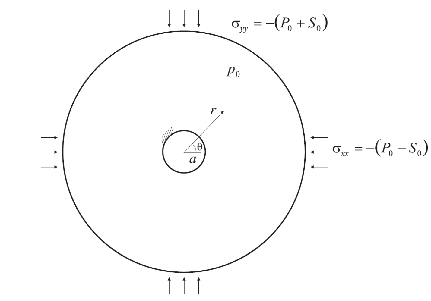
Figure 1: Problem definition.

For this problem, the initial conditions are characterized by an in-situ pore pressure (\(p_0\)) = 1 MPa, an in-situ isotropic stress (\(P_0\)) = 3 MPa, and an in-situ deviatoric stress (\(S_0\)) = 1 MPa. The following material properties are prescribed.

shear modulus (\(G\))	1.5 × 109 Pa
bulk modulus (\(K\))	1.5 × 109 Pa
porosity (\(n\))	0.3
Biot coefficient (\(α\))	0.65
Biot modulus, fluid (\(M\))	2.0 × 109 Pa
permeability (\(k\))	10-12 (m/sec)/(Pa/m)

Closed-Form Solution

The two-dimensional poroelastic solution for a borehole in a non-hydrostatic stress field can be found in Detournay and Cheng (1988). The general solution is derived in the Laplace transform domain. Results in the time domain can be obtained using a numerical inversion technique. The short-time asymptotic solution for the region near the borehole is also presented. This solution is formulated by superposition of asymptotic solutions for three loading modes: (1) a far-field isotropic stress; (2) an initial pore-pressure distribution; and (3) a far-field stress deviator. The stresses (\(σ_{rr}, , σ_{θθ} , σ_{rθ}\)), pore pressure (\(p\)) and displacements (\(u_r,u_θ\)) induced by each loading mode are defined in the equations below. As shown in Figure 1, \(r\) and \(θ\) are the polar coordinates, and a is the borehole radius.

(1) Loading Mode 1: Far-Field Isotropic Stress

This loading mode produces the classical Lamé solution in elasticity. The rock deformation is entirely associated with the deviatoric strain, and there is no mechanism for pore pressure generation. Also, the stress field and displacements are independent of the bulk modulus of the rock and of time.

\[\eqalignno{ \sigma_{rr} &=\ - P_0 (1 - {{a^{2}}\over{r^{2}}}) \cr \sigma_{\theta \theta} &=\ - P_0 (1 + {{a^{2}}\over{r^{2}}}) \cr \cr \sigma_{r \theta} &=\ 0 \cr \ \ \ & &\ \ \cr u_r &=\ - {{P_0}\over{2G}} {{a^{2}}\over{r}} \cr \cr u_{\theta} &=\ 0 \cr \cr p &=\ 0 }\]

(2) Loading Mode 2: Initial Pore Pressure Distribution

The short-time asymptotic solution for stresses, pore pressure and displacements are given:

\[ \begin{align}\begin{aligned}\eqalign{\sigma_{rr} &= -2 \eta p_0 \left\{{\left({a}\over{r}\right)}^{{3}\over{2}} \left[ \sqrt{{4 c t}\over{a^2 \pi}} \exp \left( -{{{(r-a)}^2}\over{4 c t}} \right) - \left( {{r}\over{a}} - 1 \right) \hbox{erfc} \left( {{r - a}\over{\sqrt{4 c t}}} \right) \right] - {{a^2}\over{r^2}} \sqrt{{4 c t}\over{a^2 \pi}} \right\} \cr\\\sigma_{\theta \theta } &= 2 \eta p_0 \left\{{\left({a}\over{r}\right)}^{{3}\over{2}} \left[ \sqrt{{4 c t}\over{a^2 \pi}} \exp \left( -{{{(r-a)}^2}\over{4 c t}} \right) + \hbox{erfc} \left( {{r - a}\over{\sqrt{4 c t}}} \right) \right] - {{a^2}\over{r^2}} \sqrt{{4 c t}\over{a^2 \pi}} \right\}\\&+\ \ \ \ \ \ \ 2 \eta p_0 \left\{{{{1}\over{8}} \sqrt{{{a}\over{r}}} \left( 1 - {{a}\over{r}} \right) \left[ \sqrt{{4 c t}\over{a^2 \pi}} \ \exp \left( -{{{(r-a)}^2}\over{4 c t}} \right) - \left( {{r}\over{a}} - 1 \right) \hbox{erfc} \left( {{r - a}\over{\sqrt{4 c t}}} \right) \right] } \right\} \cr\\\sigma_{r \theta} &= 0 \cr\\u_r &= 2 \eta {{a p_0}\over{2G}} \left\{\sqrt{{a}\over{r}} \left[ \sqrt{{4 c t}\over{a^2 \pi}} \ \exp \left( -{{{(r-a)}^2}\over{4 c t}} \right) - \left( {{r}\over{a}} - 1 \right) \hbox{erfc} \left( {{r - a}\over{\sqrt{4 c t}}} \right) \right] + {{a}\over{r}} \sqrt{{4 c t}\over{a^2 \pi}} \right\} \cr\\u_{\theta} &= 0 \cr\\p\over{p_0} &= 1 - \sqrt{{{a}\over{r}}} \ \hbox{erfc} \left( {{r - a}\over{\sqrt{4 c t}}} \right) - {{1}\over{8}} \sqrt{{{a}\over{r}}} \left( 1 - {{a}\over{r}} \right)\\&\times\ \ \ \ \ \ \ \left[ \sqrt{{4 c t}\over{a^2 \pi}} \ \exp \left( -{{{(r-a)}^2}\over{4 c t}} \right) - \left( {{r}\over{a}} - 1 \right) \hbox{erfc} \left( {{r - a}\over{\sqrt{4 c t}}} \right) \right]\\}\end{aligned}\end{align} \]

The poroelastic coefficient, \(η\), and the diffusivity, \(c\), involved in the above equations are defined as

\[\eta = {{\alpha (1 - 2 \nu_u)} \over {2 (1 - \nu_u)}}\]

and

\[c = k / ({1 \over M} + {{\alpha^2}\over{{K + {{4}\over{3}} G} }})\]

where \(k\) is the mobility coefficient (FLAC2D permeability), \(K\) and \(G\) are the drained bulk and shear moduli of the medium, \(M\) is the Biot modulus, \(ν\) is the drained Poisson’s ratio, and \(ν_u\) is the undrained Poisson’s ratio. The undrained Poisson’s ratio, \(ν_u\), is defined as

\[\nu_u = {{3K_u-2G}\over{2(3K_u+G)}}\]

where the undrained bulk modulus, \(K_u\), is

\[K_u = \alpha^2 M + K\]

The mode 2 solution indicates that a maximum tensile stress \(σ_θθ=2ƞp_0\) is reached at the borehole wall.

(3) Loading Mode 3: Far-Field Deviator

The mode 3 solution is for deviatoric loading. The following short-time asymptotic equations for stresses, pore pressure and displacements are obtained for this mode:

\[\eqalignno{ \sigma_{rr} &=\ S_0 \left[ 1 - 4 {{a^2}\over{r^2}} +3 {{a^4}\over{r^4}} \right] \cos 2 \theta \cr \cr \cr \sigma_{\theta \theta} &=\ S_0 \left[ -1 + 4 {{\nu_u - \nu}\over{1 - \nu}} \sqrt{{{a}\over{r}}} \hbox{erfc} \left( {{r - a}\over{\sqrt{4 c t}}} \right) -3 {{a^4}\over{r^4}} \right] \cos 2 \theta \cr \cr \cr \sigma_{r \theta} &=\ S_0 \left[ -1 - 2 {{a^2}\over{r^2}} +3 {{a^4}\over{r^4}} \right] \sin 2 \theta \cr \ \ \ & &\ \ \cr u_r &=\ {{a S_0}\over{2G}} \left[ 4(1-\nu_u) {{a}\over{r}} - {{a^3}\over{r^3}} \right] \cos 2 \theta \cr \cr \cr u_{\theta} &=\ {{a S_0}\over{2G}} \left[ -2(1-2 \nu_u) {{a}\over{r}} - {{a^3}\over{r^3}} \right] \sin 2 \theta \cr \cr \cr p &=\ S_0 {{4}\over{3}} B(1+\nu_u) \left[ -\sqrt{{{a}\over{r}}} \hbox{erfc} \left( {{r - a}\over{\sqrt{4 c t}}} \right) + {{a^2}\over{r^2}} \right] \cos 2 \theta \cr }\]

In the mode 3 equations, the Skempton coefficient, \(B\), is expressed as

\[B = (K_u - K)/ (\alpha K_u)\]

The superposition of the three loading mode solutions is performed in three FISH functions “stor_pp”, “stor_sigt” and “stor_ur” to provide solutions for pore pressure, tangential stress and radial displacement, respectively, for comparison to the FLAC2D results. Note that the FISH function “ERFC.FIS” is used to calculate the complementary error function.

Model

The FLAC2D grid used in the simulation is shown in Figure 2. The model takes advantage of the problem quarter symmetry: it corresponds to a quarter of a ring with inner radius a equal to 1 m, and outer radius b equal to 50 m. The origin of the system-of-reference axes is at the borehole center; the \(x\)- and \(y\)-axes are in the direction of the minimum and maximum compressive in-situ principal stresses, respectively. The boundary conditions correspond to roller boundaries along the symmetry lines, zero pore pressure and no traction at the borehole, and fixed displacements at the far boundary. The grid has 50 zones in the radial direction and 16 zones on the circumference, The radial extent of the model is selected such that the stress state at the outer boundary, estimated using the Kirsch solution, compares with good accuracy to the in-situ stress field.

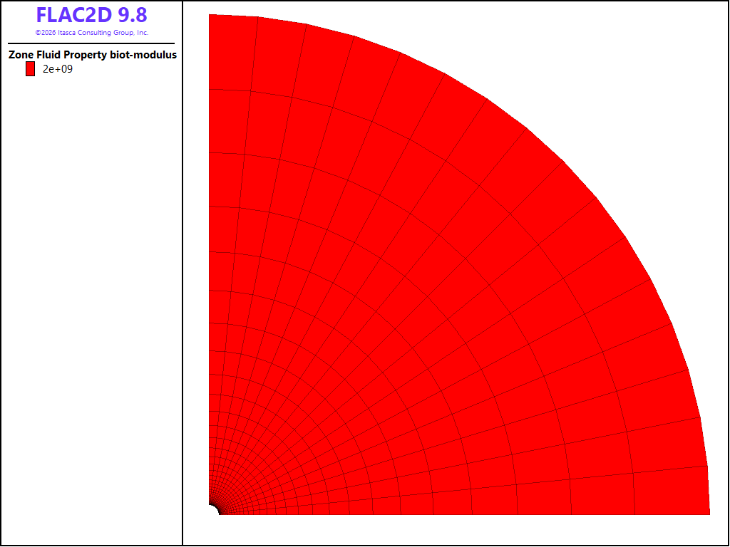
Figure 2: FLAC2D grid.

To qualify as a short-time simulation, the total simulation time must correspond to a value of the normalized time \(t^*=ct/a^2\) smaller than \(10^{-2}\) (see Detournay and Cheng 1988). The selected target time, \(t^*\) , of approximately \(10^{-3}\) is well within the range of applicability of the short-time asymptotic solution. With a diffusivity, \(c\), for this problem of approximately \(2 × 10^{-3}\) m²/s, and a borehole radius of 1 m, this time translates to roughly 0.5 second. The magnitude of the radius of influence of the borehole at that time is estimated, using \(R =\sqrt{4ct}\), at roughly 0.1 m. The grid is graded in the radial direction with a ratio of 1.18, so that 15 zones cover the radius of influence. (Note that the total number of zones in the radial and tangential directions must be large enough for the zone aspect ratio to remain below approximately 5:1 in order to avoid numerical inaccuracies.) The FLA2D model is run to three times: \(t\) = 0.003 s, 0.03 s and 0.3 s. These times correspond to normalized times \(t^*=0.7×10^{-5}\), \(0.7×10^{-4}\) and \(0.7×10^{-3}\) respectively. The analytical and FLAC2D results for pore pressure, tangential stress and radial displacement are stored in tables.

The simultion is run in two different ways. First, fully coupled, where a single fluid timestep is taken and mechanical solves to equilibrium for each fluid step. This is shown in the data file borehole.dat. The second approach, shown in borehole_uncoupled.dat in an uncoupled approach where fluid solves to a specified time, followed by solving to mechanical equilibrium. In this case, fluid modulus needs to be adjusted to account for the lack of storativity in the fluid-only solution (see zone fluid modulus-scale). Also, the generation of pore pressure during the mechanical solution is turned off with zone fluid property pore-pressure-generation off.

Results and Discussion

The results and discussion of the FLAC2D simulation closely follow those in Detournay and Cheng (1988). Results of the coupled and uncoupled simulations are very similar. The main difference between the two solutions is that the uncoupled approach solves more quickly. Figures below show results from the coupled simulation.

Isochrones of pore pressure variation with radius are compared to the analytical solution in Figure 3 for \(t\) = 0.003 s, 0.03 s, 0.3 s, and the direction \(θ\) = 0. The steep radial gradient of pore pressure developing at the borehole wall is illustrated in this figure. This gradient is associated with a rapid drainage of fluid near the borehole, which influences the apparent stiffness properties of the rock.

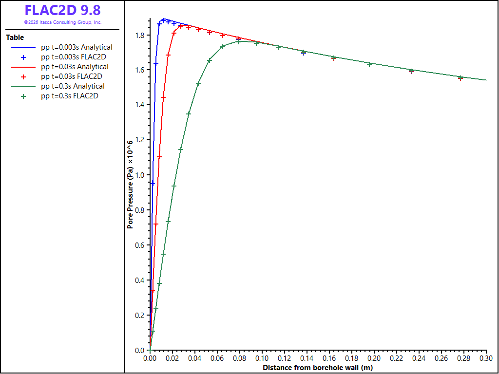
Figure 3: Pore pressure variation with radius at \(θ\) =0° (\(t\) =0.003s, 0.03s and 0.3s).

The drained modulus characterizes the rock in the vicinity of the borehole, and the stiffer undrained modulus characterizes the rock farther away. The shielding effect on the stress concentration near the borehole caused by this stiffness contrast is shown in Figure 4. In this figure, the isochrones of tangential stress variation with radius are compared to the analytical solution for the three values of time considered earlier and along the \(x\)-direction. As this figure shows, at the very small times considered in the simulation, the peak tangential stress is actually located inside the rock. This mechanism explains field observations that indicate that failure can be initiated at a small distance inside the rock, rather than at the borehole wall as predicted by an elastic analysis.

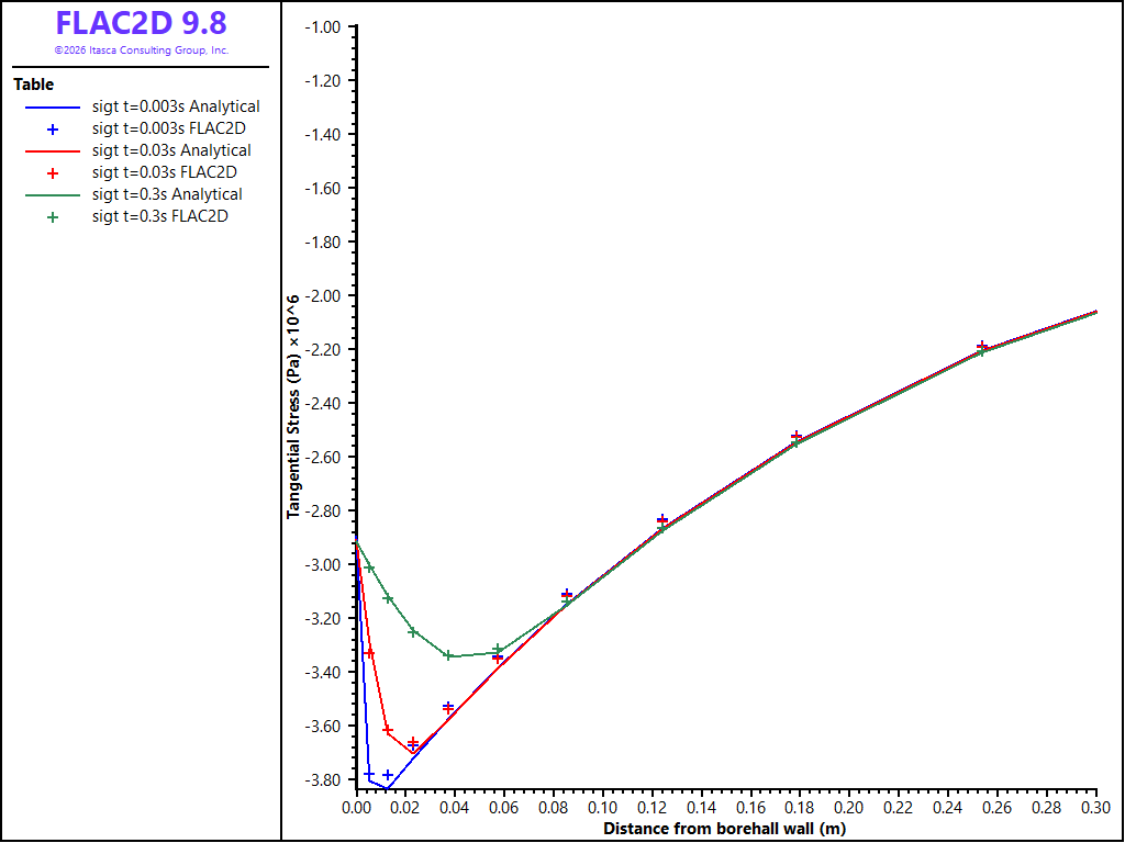
Figure 4: Tangential stress variation with radius at \(θ\) =0° (\(t\) =0.003s, 0.03s and 0.3s).

The radial displacement versus θ is compared to the analytical solution in Figure 5 for a simulation time of 0.3 second. The results of the FLAC2D simulation show good agreement with the analytical predictions.

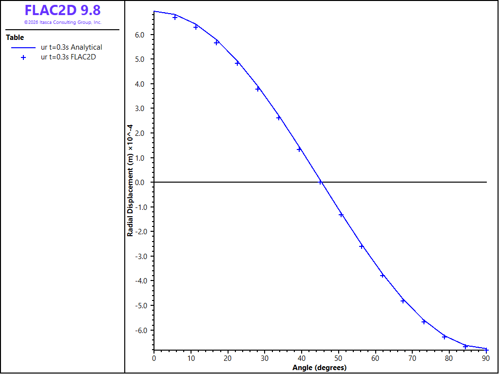
Figure 5: Radial displacement variation with \(θ\) at \(r=a\) (\(t\) =0.3s).

References

Detournay, E., and A. H.-D. Cheng. “Poroelastic Response of a Borehole in a Non-Hydrostatic Stress Field,” Int. J. Rock Mech. Min. Sci. & Geomech. Abstr., 25(3), 171-182 (1988).

Data Files

borehole.dat

;---------------------------------------------------------------------
;;; Poroelastic Response of a Borehole
;---------------------------------------------------------------------
model new
model large-strain off
fish automatic-create off
model deterministic on
model title "Poroelastic Response of a Borehole"
model configure fluid-flow

; from FLAC 8.1
;zone import 'radial'

zone create2d annular-sector point 0 0,0 point 1 50,0 point 2 0,50 ...
  point 3 1,0 point 4 0,1 size 50 16 ratio 1.18 1

program call 'Erfc.fis' suppress
program call 'fishfunctions.dat' suppress
zone face skin
zone cmodel assign elastic

; --- properties ---
zone property bulk [c_bu] shear [c_sh] density 2500

;fluid properties
zone fluid property porosity [c_n] mobility-coefficient [c_k] 
zone fluid property biot-coefficient [c_bc] biot-modulus [c_bm]
zone fluid property fluid-density 1000 
zone fluid property pore-pressure-generation on
zone fluid unsaturated cutoff 

; boundary conditions
zone gridpoint fix velocity-x range group 'West2'
zone gridpoint fix velocity-x range group 'East'
zone gridpoint fix velocity-y range group 'East'
zone gridpoint fix velocity-y range group 'Bottom

; initial conditions
zone initialize stress xx [sxx0] yy [syy0] zz [sxx0]
zone gridpoint initialize pore-pressure [pp0]

; --- undrained response ---
model solve-static
model save 'bh_a'

; --- drained response ---
zone face apply pore-pressure 0 range group 'West1'
model fluid timestep fix 3e-4

model solve-fluid-coupled fluid time-total 3e-3
[stor_pp('pp t=0.003s')]
[stor_sigt('sigt t=0.003s')]
model save 'bh1'

model solve-fluid-coupled fluid time-total 3e-2
[stor_pp('pp t=0.03s')]
[stor_sigt('sigt t=0.03s')]
model save 'bh2'

model solve-fluid-coupled fluid time-total 3e-1
[stor_pp('pp t=0.3s')]
[stor_sigt('sigt t=0.3s')]
[stor_ur('ur t=0.3s')]
model save 'bh3'

borehole_uncoupled.dat

model restore 'bh_a'

; --- drained response ---
zone face apply pore-pressure 0 range group 'West1'
model fluid timestep fix 3e-4

; automatically calculates modulus 
; for fluid-only analysis (=c_bma)
zone fluid modulus-scale 

model solve-fluid time-total 3e-3

; turn off generation of pore pressures with volumetric changes
zone fluid property pore-pressure-generation off
model solve-static
[stor_pp('pp t=0.003s')]
[stor_sigt('sigt t=0.003s')]
model save 'bh1-uc'

;
model solve-fluid time-total 3e-2

model solve-static

[stor_pp('pp t=0.03s')]
[stor_sigt('sigt t=0.03s')]
model save 'bh2-uc'

model solve-fluid time-total 3e-1

model solve-static

[stor_pp('pp t=0.3s')]
[stor_sigt('sigt t=0.3s')]
[stor_ur('ur t=0.3s')]
model save 'bh3-uc'

Endnote

[1]

This example is listed under the present document title in the i Examples dialog (use the menu command Help -> Examples… to access).