Infinite Line Heat Source in an Infinite Medium (FLAC2D)

Verification Problem

The project file for this example may be viewed/run in FLAC2D.[1] The main data file used is shown at the end of this example.

How To Read and Use Examples

An infinite line heat source with a constant heat-generating rate is located in an infinite elastic medium with constant thermal properties. Nowacki (1962) provides the solution to this problem for the transient values of temperature, radial and tangential stress, and radial displacement:

(1)\[\begin{split}\begin{split} {{T}\over{a}}\ &=\ {1 \over {4 \pi}}\ E_1\ \left( \xi \right) \\ {{\sigma_r}\over{bG}}\ &=\ {1 \over {-4 \pi}}\ \left[ E_1 \left( \xi \right) + {{1 - e^{- \xi}} \over {\xi}} \right] \\ {{\sigma_t}\over{bG}}\ &=\ {1 \over {-4 \pi}}\ \left[ E_1 \left( \xi \right) - {{1 - e^{- \xi}} \over {\xi}} \right] \\ {{u_r}\over{bL}}\ &=\ {1 \over {8 \pi}}\ r \ \left[ E_1 \left( \xi \right) + {{1 - e^{- \xi}} \over {\xi}} \right] \end{split}\end{split}\]

where:	\(\xi\)	= \({r^2}\over{4 \kappa t}\);
	\(r\)	= radial distance to the line source;
	\(\kappa\)	= \({k \over {\rho C_p}}\);
	\(a\)	= \({q \over {k}}\);
	\(b\)	= \(\alpha_t \ a {9 K \over {3K + 4G}}\);
	\(L\)	= unit length;
	\(q\)	= energy uniform per unit length; and
	\(E_1(\xi)\)	= \(\int_{\xi}^\infty {e^{-u} \over {u}} du\) is the exponential integral.

The material properties and initial and boundary conditions for this example are defined as follows:

Material Properties
density (\(\rho\))	2000 kg/m3
specific heat (\(C_p\))	1000 J/kg °C
thermal conductivity (\(k\))	4 W/m °C
linear thermal-expansion coefficient (\(\alpha_t\))	5 × 10-6/ °C
shear modulus (\(G\))	30 GPa
bulk modulus (\(K\))	50 GPa
Initial/Boundary Conditions
initial uniform temperature	0°C
initial stress state	no stresses
Line Heat Source
energy release per unit length (\(q\))	1600 W/m

It is assumed that the material properties are temperature-independent, the thermal output of the source is constant (no decay), and the line heat source is of infinite length.

The FLAC2D grid for this problem is a quarter-section of a cylindrical disk. The axis of the line heat source coincides with the y-axis of the model. The grid is radially graded in the xy-plane. The model is shown in Figure 1.

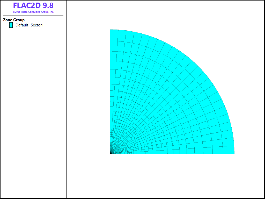
Figure 1: FLAC2D grid for an infinite line heat source.

The line heat source is represented in FLAC2D by a point source. For a quarter-symmetry model, the intensity of the point source \(q_p\) is adjusted to produce an energy release equivalent to that of a line source of linear intensity \(q\) into the model. the relation between \(q_p\) and \(q\) is

(2)\[q_p\ =\ {q L \over 4}\]

The constant point heat source is applied at gridpoints along the z-axis; the boundaries of the model are kept adiabatic to represent thermal symmetry planes. the boundaries along the x-axis and y-axis are fixed to represent shear-free symmetry planes.

An uncoupled analysis is recommended because the material is elastic. The problem is first thermally solved to an age of one year and then stepped to mechanical equilibrium.

The dimensionless form of the analytical solutions in the equations above are programmed via FISH functions. The analytical and numerical values can then be compared directly in tables. The analytical solutions for temperature and radial displacement are programmed in the FISH function ana_soltu, and for radial and tangential stresses in ana_solst. The exponential integral function used in the analytical solutions is programmed as a separate FISH function called exp-int. The dimensionless values for the numerical results for temperature and displacement are calculated in the FISH function num_soltu, and for radial and tangential stresses in num_solst. The numerical values for dimensionless temperature, radial stress, tangential stress, and radial displacement are stored in Tables 1, 3, 5, and 7, respectively. The analytical values for dimensionless temperature, radial stress, tangential stress, and radial displacement are stored in Tables 2, 4, 6, and 8, respectively.

The results for temperature, radial displacement, and radial and tangential stress distributions at 1 year are presented in the table plots in Figure 2 to Figure 4. The difference between numerical and analytical solutions for temperature is less than 2%. The comparison is also good for displacements and for stresses; the difference is generally less than 2% within 100 m of the heat source. The fixed outer boundary has an influence on the numerical results farther from the source, but the agreement is still reasonable.

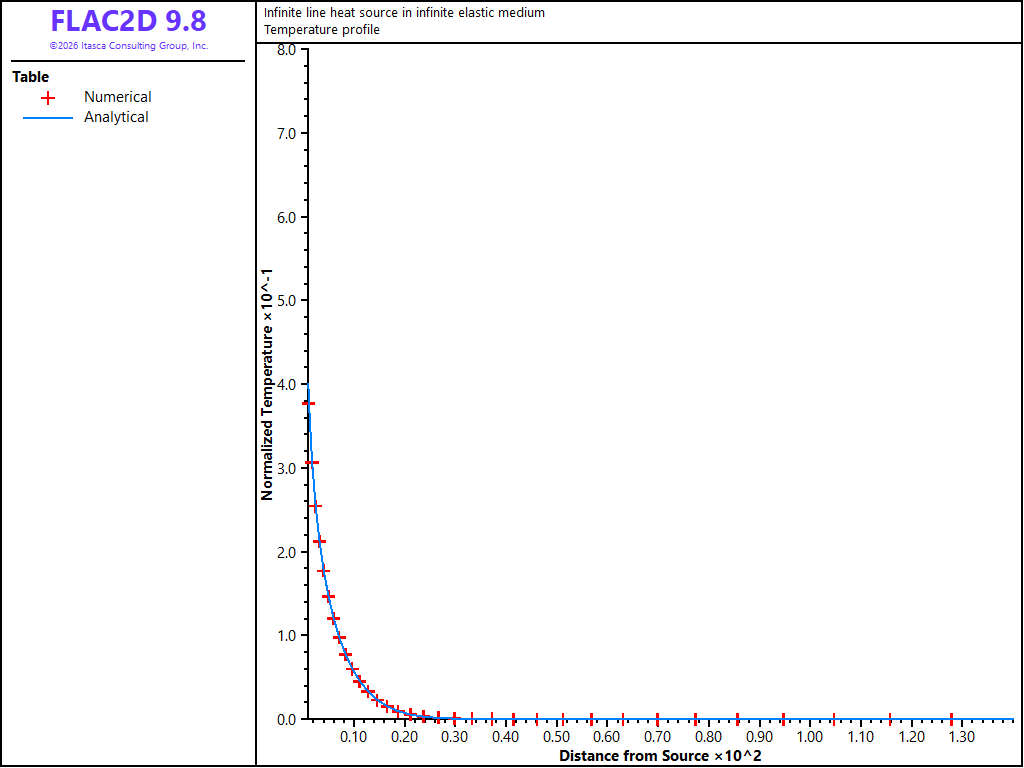
Figure 2: Temperature distribution at 1 year.

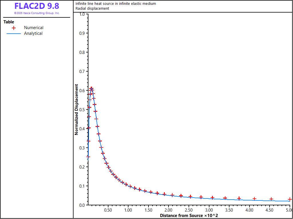
Figure 3: Radial displacement distribution at 1 year.

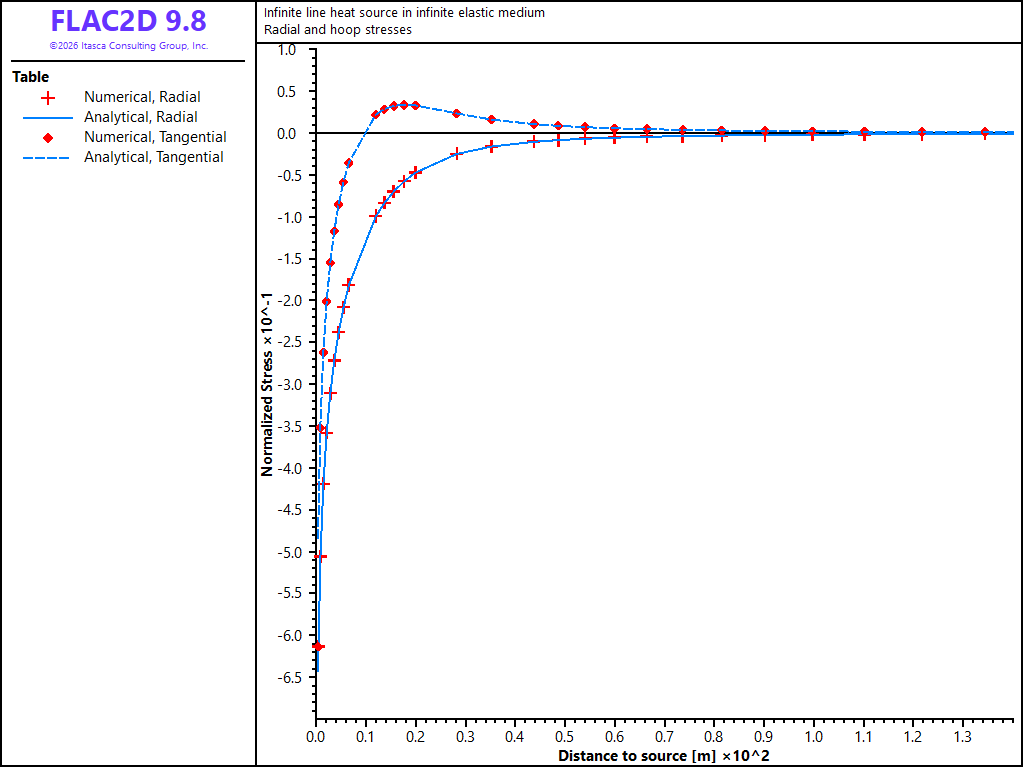
Figure 4: Radial and tangential stress distributions at 1 year.

Reference

Nowacki, W. Thermoelasticity. New York: Addison-Wesley (1962).

Data File

model new
model title 'Infinite line heat source in infinite elastic medium'
;--- model geometry
zone create sector point 1 (500,0) point 2 (0,500) size (48,24) ratio (1.1,1)
zone face skin
zone face group 'Out' range group 'East'
; --- mechanical model
model large-strain off
zone nodal-mixed-discretization off
zone cmodel assign elastic
zone property density 2e3 bulk 5e10 shear 3e10
zone face apply velocity-x 0 range group 'West'
zone face apply velocity-y 0 range group 'Bottom'
; --- thermal model
model configure thermal
zone thermal property conductivity 4 expansion 5e-6 specific-heat 1e3
; --- line source
zone gridpoint fix source 400 range position-x 0 position-y 0
model save 'line-year0'

;  uncoupled analysis
model solve-thermal time-total [365*24*60*60]
model solve-static
model save 'line-year1-ucpl'

Endnote

[1]

This example is listed under the present document title in the i Examples dialog (use the menu command Help -> Examples… to access).