Transient Fluid Flow to a Well in a Shallow Confined Aquifer (FLAC2D)

Note

The project file for this example is available to be viewed/run in FLAC2D. The project’s main data files are shown at the end of this example.

Problem Statement

A shallow confined aquifer of large horizontal extent is characterized by a uniform initial pore pressure, \(p_0\), and initial isotropic stress, \(\sigma_0\). A well, fully penetrating the aquifer, is producing water at a constant rate, \(Q\), from time, \(t = t_0\). The elastic porous medium is homogeneous and isotropic, and the flow of groundwater is governed by Darcy’s law. Transient effects are linked to the compressibility of water and the soil matrix. In this problem, the effect of pore-pressure changes on stresses is small compared to the pressure of the overburden, and the vertical stress in the aquifer may be assumed to remain constant with time. Also, horizontal strains are neglected because they are small compared to vertical strains. The problem is axisymmetric. The conditions of fluid flow to the well are illustrated schematically in Figure 1

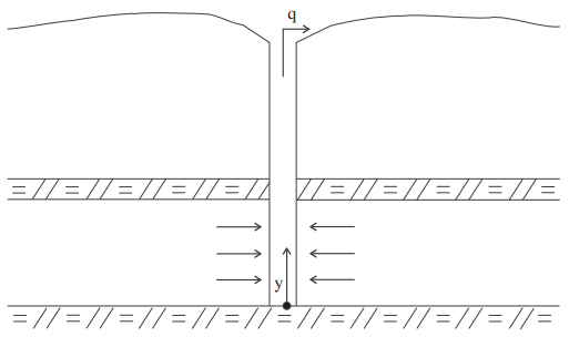
Figure 1: Flow to a well in a shallow confined aquifer.

The properties for this example are defined:

shear modulus (\(G\))	71 MPa
bulk modulus (\(K\))	118 MPa
water bulk modulus (\(K_w\))	2 GPa
porosity (\(n\))	0.4
mobility coefficient (\(\lambda\))	2.98 × 10-8 \({m^2}\over{Pa-sec}\)

The initial pore pressure is 220 kPa and the initial isotropic stress is 147 kPa. The well pumping rate per unit aquifer thickness, is 2.21 × 10^-3 \({m^2}\over{s}\), and the well radius, \(r_w\), is selected as 1 m.

Analytical Solution

A cylindrical system of coordinates is considered with the \(y\)-axis pointing upward and aligned with the well axis. Substitution of the transport law in the fluid mass-balance equation gives, for incompressible grains, and taking into consideration that horizontal strains are zero (:math::\(\varepsilon_{rr}=\varepsilon_{\theta \theta} = 0\)):

(1)\[\frac{n}{K_w}\frac{\partial p}{\partial t} - \lambda \nabla^2 p = - \frac{\partial \varepsilon_{yy}}{\partial t}\]

where \(\lambda\) is the mobility coefficient, \(K_w\) is the water bulk modulus, \(n\) is the porosity, \(\varepsilon_{yy}\) is the vertical strain, and \(p\) is the pore pressure. Partial differentiation with respect to time of the elastic constitutive relation \(\left(\sigma_{yy}-\sigma_0\right) + \left(p - p_0 \right) = \alpha_1\varepsilon_{yy}\) yields, for constant vertical stress:

(2)\[\frac{\partial p}{\partial t} = \alpha_{1} \frac{\partial \varepsilon_{yy}}{\partial t}\]

where the confined modulus is \(\alpha_1=K+4G/3\). Using the last equation to express \(\varepsilon_{yy}\) in terms of \(p\), we obtain, after some manipulation:

(3)\[\frac{\partial p}{\partial t} = c \nabla^2 p\]

where \(c=\lambda M\) is the consolidation coefficient and \(M = \left(n/K_w + 1/\alpha_1 \right)^{-1}\) is the Biot modulus. Because the problem is axisymmetric and not dependent on \(y\), the Laplacian of pore pressure can be expressed as:

(4)\[\nabla^2 p = \frac{\partial^2 p}{\partial r^2} + \frac{1}{r} \frac{\partial p}{\partial r}\]

The solution to this differential equation with boundary conditions:

(5)\[\begin{split}\begin{split} p \vert_{r=\infty} &= p_0 \\ \frac{\partial p}{\partial r} \vert_{r=r_w} &= - \frac{Q}{2 \pi r_w \lambda} \end{split}\end{split}\]

is given by Theis (1935). It has the form:

(6)\[\hat{p} = -\frac{1}{4\pi} \mathrm{E}_{1} \left(\frac{r^2}{4ct}\right) + \hat{p}_0\]

where \(\hat{p}=p\lambda/Q\) is a dimensionless pressure and \(E_1\) is the exponential integral, defined as:

(7)\[\mathrm{E}_{1} \left(u\right) = \int_{u}^{\infty} \frac{e^{-\xi}}{\xi} d\xi\]

The vertical displacement may be obtained by integration of the equilibrium equation, \(\partial \sigma_{yy}/\partial y = 0\), after expressing \(\sigma_{yy}\) in terms of \(\varepsilon_{yy}\) by means of the mechanical constitutive equation, and substitutivg \(\partial \varepsilon_{yy}/\partial y\) for \(\varepsilon_{yy}\). This yields, after substitution of the boundary condition and using the above solution for pore pressure:

(8)\[\hat{u}_y = -\frac{\hat{y}}{4\pi}E_{1} \left(u\right)\]

where \(\hat{u}_y = u_y \lambda \alpha_{1} / Q\) is a dimensionless vertical displacement, \(\hat{y} = y / H\) is a dimensionless vertical coordinate.

The stresses are derived from the mechanical constitutive equation and the solution for pore pressure. They have the form:

(9)\[\begin{split}\begin{split} \hat{\sigma}_{rr} &= \hat{\sigma}_{\theta \theta} = \frac{1}{2\pi} E_{1} \left(u\right) + \hat{\sigma}_0 \\ \hat{\sigma}_{yy} &= \hat{\sigma}_0 \end{split}\end{split}\]

where \(\hat{\sigma}=\sigma\lambda \alpha_{1}/\left(QG\right)\).

Results

The FLAC2D fluid flow model is run in axisymmetric mode, given by the commands model configure fluid-flow and model configure axisymmetry. The axis of symmetry is at the well axis at \(x=0\), and a slice of unit thickness of the aquifer is modeled. The far boundary of the flow domain is located 100 m from the well axis.

In total, 50 zones are used, aligned and graded in the radial direction. The displacements are fixed in the radial direction and in the vertical direction at the base of the model. A vertical pressure of magnitude \(\sigma_0\) is applied at the top of the model.

Stresses and pore pressures are initialized to the values given above. The well flow rate is constant and modeled as a discharge of magnitude \(Q/\left(2\pi r_w\right)\), applied at the well radius, \(r=r_w\).

The problem is solved using the model solve-fluid-decoupled command. This example is pore pressure driven, and the value of the stiffness ratio is approximately 23. Thus, the flow calculation may be uncoupled from the mechanical calculation. The fluid modulus during the flow-only step is scaled using zone fluid modulus-scale in order to preserve the diffusivity of the system. The problem is solved for a total of 32 seconds.

The analytical solution for pore pressure, stresses, and vertical displacement are programmed as a FISH function. Analytical and numerical values are stored in tables. The results are then compared in graphical form below. By convention, in the figures, lines correspond to the analytical solutions and crosses to the numerical results.

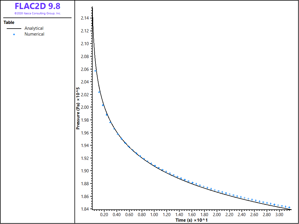
Figure 2: Well pressure history at the well radius.

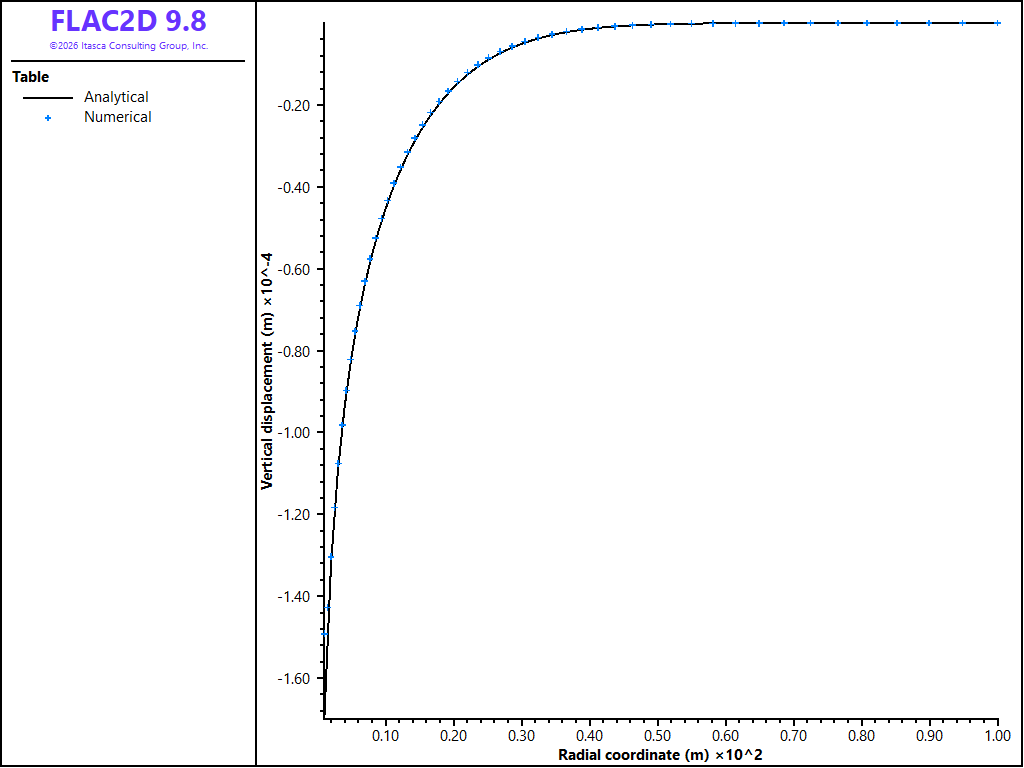
Figure 3: Vertical displacement profile at 32 seconds.

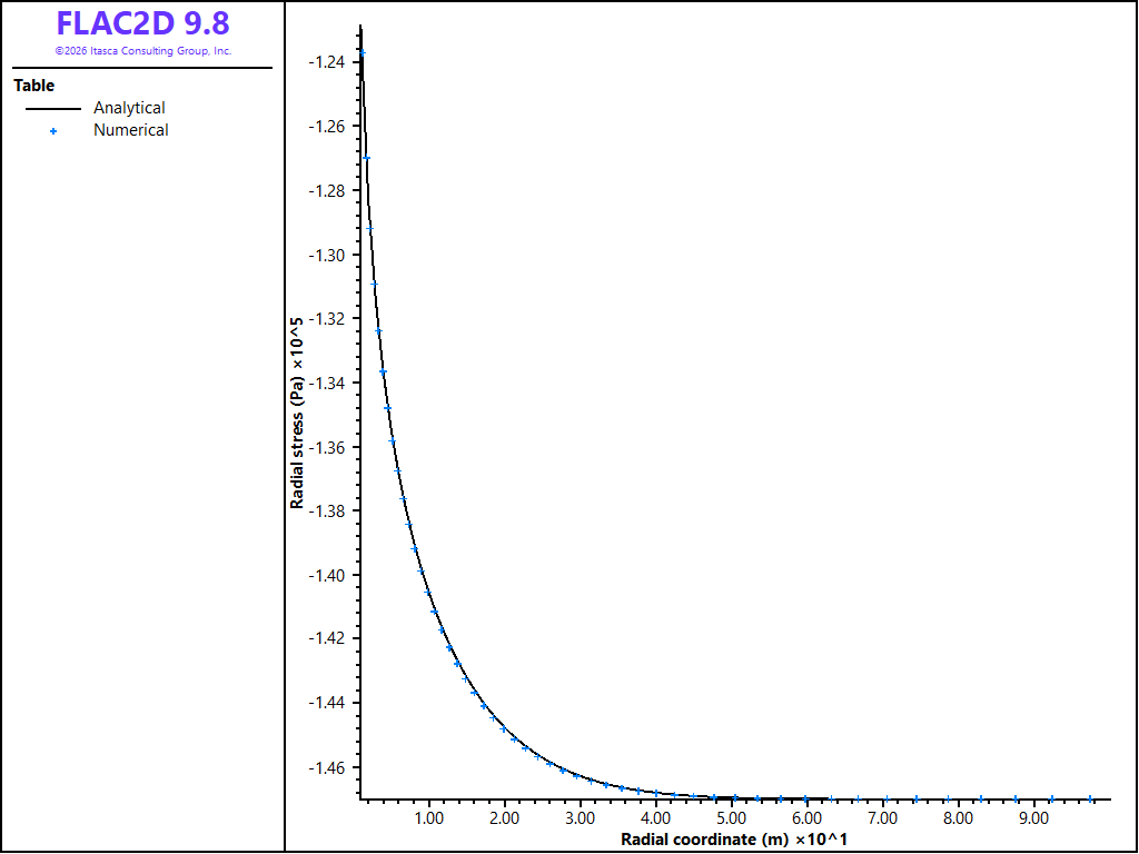
Figure 4: Radial stress profile at 32 seconds.

Reference

Theis, C. V. “The Relation between the Lowering of the Piezometric Surface and the Rate and Duration of Discharge of a Well Using Groundwater Storage,” Trans. Am. Geophys. Union, 10, 519-524 (1935).

Data File

radialflowtowell.dat

model new
model configure fluid-flow axisymmetry
model large-strain off

; Model parameters
[pi = 220e3]     ; Initial pressure
[Q  = 2.21e-3]   ; Production rate (m^2/s)
[n = 0.40]       ; Porosity (-)
[K = 118e6]      ; Bulk modulus (Pa)
[G = 71e6]       ; Shear modulus (Pa)
[Kw = 2e9]       ; Water bulk modulus (Pa)
[mob = 2.98e-8]  ; Mobility (m^2/(Pa*s))
[rw  = 1.0]      ; Well radius (m)
[re  = 100]      ; Far field radius (m)

; Model geometry
zone create quadrilateral point 0 ([rw],0) point 1 ([re],0) ...
    point 2 ([rw],1) point 3 ([re],1) size 50 1 ratio 1.05
zone face skin

; Mechanical model
zone cmodel assign elastic
zone property bulk [K] shear [G]

zone gridpoint fix velocity-x
zone face apply velocity-y 0 range position-y 0

zone initialize stress xx -1.47e5 yy -1.47e5 zz -1.47e5
zone face apply stress-normal -1.47e5 range position-y 1

; Fluid flow model
zone fluid property mobility-coefficient [mob]
zone fluid property porosity [n] fluid-modulus [Kw]
zone fluid modulus-scale

zone gridpoint initialize pore-pressure [pi]
zone face apply discharge [-Q/(2*math.pi*rw)] range group 'Skin=West'

; Well pressure history
[counter = 1]
fish define track_well_press
    local gp = gp.near(rw,0.0)
    table.x("num_p",counter) = fluid.time.total
    table.y("num_p",counter) = gp.pp(gp)
    counter += 1
end

; Solve decoupled
fish callback add [track_well_press] -1 interval 50 process fluid
model solve-fluid-decoupled time 32.0 stages 2