Visualizing the Results

MINEDW offers multiple options for presenting simulation results graphically. Use “Control Panel” options to display results. Select “Node” plot items under the “List” tab in the “Control Panel” Pane to produce 2-D and 3-D contours.

2D Contour plot items: Display color floods of head, pore pressure, head difference, water table, and drawdown.

3D Contour plot items: Create 3-D contours of head, pore pressure, and head difference.

Customize display for each plot using the “Attributes” tab in the “Control Panel” Pane (MINEDW Interface). The following figures show example 2-D and 3-D plots.

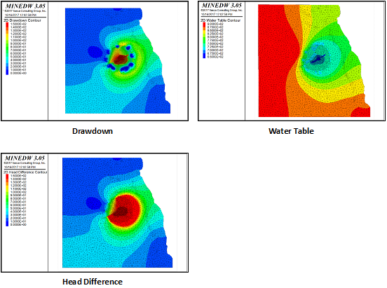
Figure 1: Sample 2-D contour plots

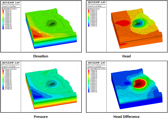
Figure 2: Sample 3-D contour plots

To create a 3-D pore-pressure plot:

1. Select the “List” tab from the “Control Panel” Pane

2. Expand the “Node” item and double-click “3D Contour” (see fig-3d-contour-attributes)

3. Select the “Attribute” tab from the “Control Panel” Pane

4. Choose “Pressure” from the “Color By” setting

5. View pore pressures in the View Pane

6. Adjust the time-step slider to view different time steps

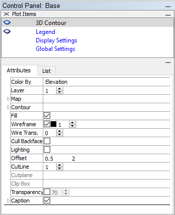
Figure 3: Attributes of the “3D Contour” plot item

To export an image of the 3-D pore-pressure plot, ensure that the desired time step is selected, then choose “Export Base” from the “File” item on the Main Menu banner and select “Bitmap.” The exported bitmap is shown in fig-head-distribution-3d.

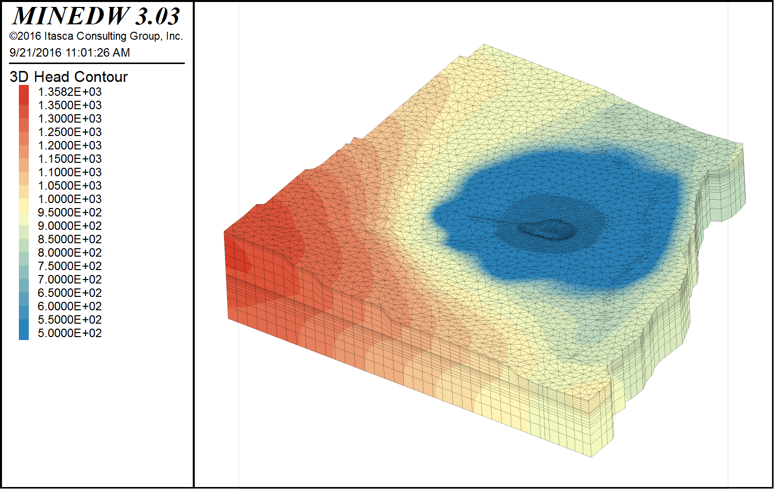
Figure 4: Screen display of head distribution in 3-D

Cross Sections

Cross sections are useful because they allow the user to visualize different types of data together at any point within the model domain. For example, a user may wish to view a cross section of the open pit showing geological units overlaid by contours of pore pressure, head, or head difference. This can be achieved by using the “3D Element,” “Isosurface,” and “Plane” plot items.

To draw a cross section, the first step is to plot the desired “3D Contour” (Elevation, Head, Pressure, or Head Difference) or “3D Element” plot item. Model geology and pore pressures are used as an example; however, similar steps can be followed to plot a cross section of any other model results.

To view model geology and pore pressures, select the “List” tab from the “Control Panel” Pane, expand the “Element” item, and double-click “3D Element.” Now, add an “Isosurface” plot item (be sure to import results) by expanding the “Node” item and double-clicking “Isosurface” (see fig-3d-element-isosurface-plot-items). On the “Attributes” tab for the “Isosurface” plot item, select “Pressure” as the “Color By” attribute. A 3-D color flood of model geology with “Isosurfaces” of pore pressures appears in the View Pane, but the “Isosurfaces” are not visible, as they are hidden by the “3D Element.” Select the desired time step to view with the time-step slider.

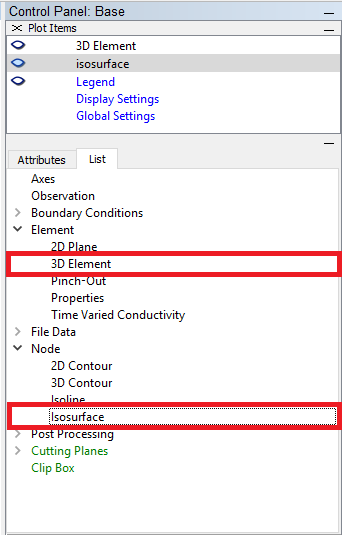
Figure 5: The “3D Element” and “Isosurface” plot items

The easiest method for creating a cross section is to use the “Plane” tool located on the Toolbar. To use it, click on it, then select two points on the displayed “3D Element” plot item. The “3D Element” and “Isosurface” plot items will be cut by a plane that passes through the two points that were selected.

Alternatively, create a cross section by selecting the “List” tab from the “Control Panel” Pane, expanding “Cutting Planes,” and double-clicking “Plane” (see fig-plane-plot-item).

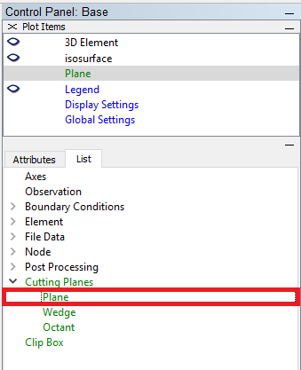
Figure 6: The “Plane” plot item

On the “Attributes” tab, define the origin, dip, and dip direction of the plane (see fig-plane-attributes).

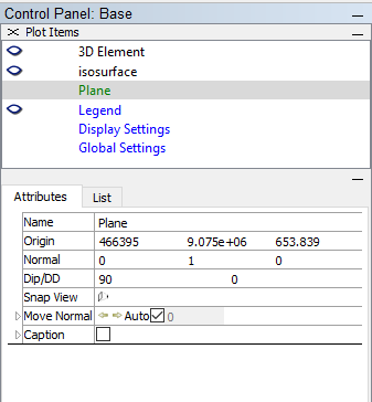
Figure 7: The attributes of the “Plane” plot item

For both methods of creating a cross section, display the front or back sections that have been cut (i.e., to turn a 2-D item into a 3-D item) by selecting “3D Element” from the list in the “Plot Items” pane and checking the box for “Front” or “Back” under “Cutplane” on the “Attributes” tab (see fig-3d-element-cutplane-attributes).

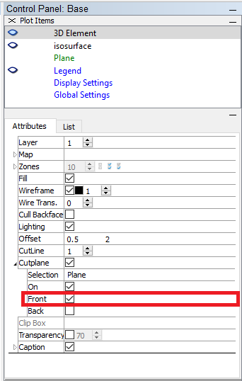
Figure 8: The attributes of the “3D Element” plot item

The cross section will display model geology through the open-pit area overlaid by contours of pore pressure (see fig-model-output-screen-display). To export the plot as a bitmap, select “Export Base” under the “File” menu and choose the “Bitmap” option.

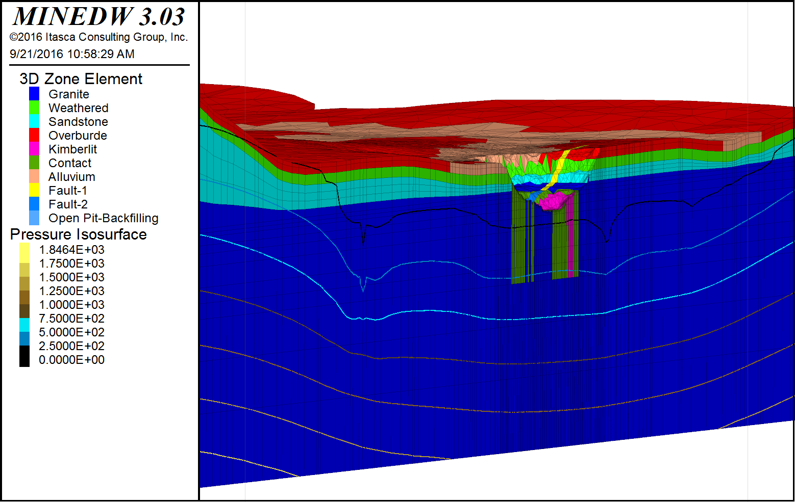
Figure 9: Screen display of output from the model run

Pit Lake – Water Level vs. Time

MINEDW computes water-level changes in pit lakes when simulated in a model. To plot pit-lake level changes over time, import the .LAK file from the folder where MINEDW was executed to Excel or other plotting software (see fig-pit-lake-water-level-time). The .LAK file also contains other useful information about the pit lake. This file contains the net flux to the pit lake as well as seepage to and from the pit lake. Evaporative losses, volume, and lake area are also recorded in this file. Note that these data are only recorded in time steps during which a pit lake is active. If seepage to the pit occurs during mining operations, it is not recorded in the .LAK file. This seepage data can be located in the .SEP file (Seepage Component to Pit).

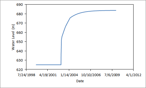
Figure 10: Pit-lake water level with time

Pumping Well – Discharge vs. Time

Pumping rates are reported in the output file with an .FLW extension. This file also contains the flux for each of the constant-head groups defined in the “Constant-Head Boundary” dialog box. The .FLW file reports extraction of groundwater from the model as negative numbers and addition of groundwater as positive numbers. Flux into or out of the model domain is reported for each time step.