Parametric Study with Python - Pseudostatic Analysis (FLAC2D)
The project file for this example may be viewed/run in FLAC2D.[1] The main data file used is shown at the end of this example.
Problem Statement
A 2D pseudostatic analysis is presented in Pseudostatic Analysis (FLAC2D). In this example, a factor-of-safety analysis is performed on a simple slope consisting of two soil layers overlaying a rigid bedrock. Only two cases were considered: a static analysis and a pseudostatic analysis, where the horizontal gravitational vector was set to an acceleration of 10% of the downward gravitational force applied to the model (\(k_h = 0.1\) and \(k_v = 0\)).
Using Python in FLAC2D, we can easily extend this to a parametric study where different slope angles and horizontal acceleration values are iterated over, and a factor-of-safety analysis is performed for each case. The input parameters and factor of safety from each case are saved, and a contour plot is generated with Matplotlib. This provides an intuitive visual representation of how factor of safety for this particular model geometry is affected by the slope angle and horizontal acceleration. WARNING: This example performs 81 factor of safety analyses and takes some time to run.
Figure 1 shows the factor-of-safety (FOS) contour plot, with a black line drawn at FOS = 1.0. The shape of the contours provides insight on how different combinations of slope angle and horizontal acceleration affect the overall stability of the slope. From the plot, we can see that increases to both the slope angle and horizontal acceleration factor cause a decrease in the FOS. However, instead of straight, diagonally oriented contours, we see a bend in each contour, depicting the point where slope angle starts to influence the stability of the slope for constant horizontal acceleration values (moving from low to high slope angles).
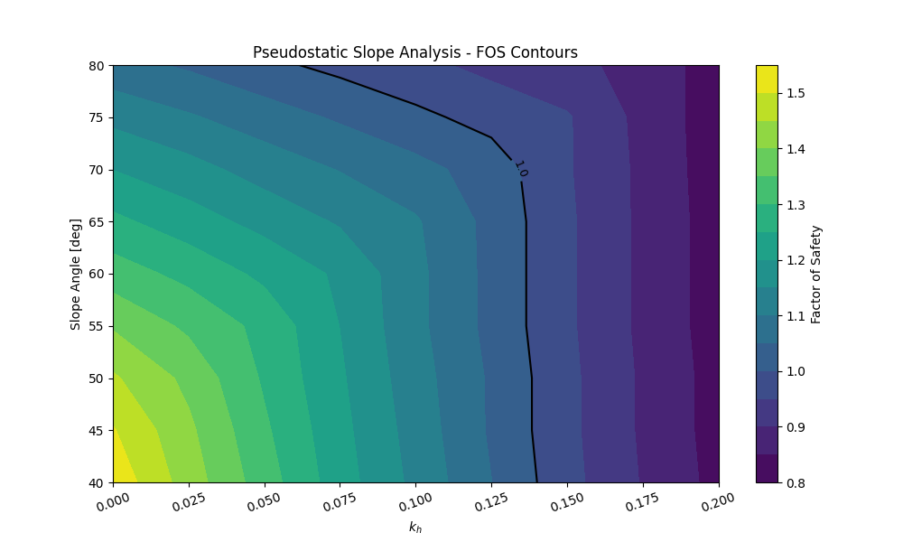
Figure 1: Factor-of-safety contour plot, as a function of slope angle and the horizontal acceleration factor \(k_h\).
Data Files
pseudostatic_study.py
import itasca as it
import numpy as np
import matplotlib.pyplot as plt

# create an empty list for storing factor of safety values for
# each slope angle
all_fos = []

# iterate over different slope angles to apply to the model
for angle in range(40, 85, 5):
    # based on the slope angle at each loop iteration, the
    # two points making up the slope face geometry are adjusted
    x1 = 10 / np.tan(np.deg2rad(angle)) + 40
    x2 = 30 / np.tan(np.deg2rad(angle)) + 40

    # the model geometry from Pseudostatic Analysis (FLAC2D)
    # is prescribed, with increased model depth and a variable
    # slope angle
    it.command(f"""
    model new
    sketch set delete

    sketch set select "slope"
    sketch edge create polyline point 0 0 0 30 40 30 40 0 40 30 220 30 40 30 {x2} 60 220 60 220 0 close
    sketch edge id 8 split (220,40)
    sketch edge id 5 split ({x1},40)
    sketch edge create by-points 9 10 type simple
    sketch block create automatic
    sketch set automatic-zone total test
    sketch set automatic-zone direction construction edge 3 min-size 1
    sketch block group "soil2" slot "Construction" range id-list 1
    sketch block group "soil1" slot "Construction" range id-list 4 2 3
    zone generate from-sketch
    model save "init_shake" compress
    """)

    # gravity is set in ft/s^2
    gravity = -32.18504

    # create an empty list for storing factor of safety values
    # for each kh value
    this_fos = []

    # iterate over different kh values to apply to the model
    # (for each slope angle)
    for kh in np.arange(0, 0.225, 0.025):
        # the model properties and boundary conditions from
        # Pseudostatic Analysis (FLAC2D) are prescribed, with
        # a variable horizontal acceleration
        it.command(f"""
        model restore "init_shake"
        model gravity ({gravity*kh}, {gravity})

        model large-strain off

        zone cmodel assign mohr-coulomb
        zone property density 3.882 bulk 2.1E6 shear 6.3E5 ...
                      cohesion 1000.0 friction 0.0 dilation 0.0 tension 1.0E10 ...
                      range group 'soil1'
        zone property density=3.416 bulk=2.088543E6 shear=6.2656E5 cohesion=600.0 ...
                      friction=0.0 dilation=0.0 tension=1.0E10 range group 'soil2'

        zone face apply velocity-x 0 range position-x 0
        zone face apply velocity-x 0 range position-x 220
        zone face apply velocity (0,0) range position-y 0

        model factor-of-safety filename 'pseudostatic'
        """)

        # append factor of safety value to list
        this_fos.append(it.fos())
    # append factor of safety list to list (creates a nested list)
    all_fos.append(this_fos)

# convert nested list of factor of safety values to a 2D numpy
# array and save it as a .npy file
all_fos = np.array(all_fos).astype(float)
np.save('fos_values_shake.npy', all_fos)

# load .npy file and create input arrays for plotting contours
# of factor of safety
all_fos = np.load('fos_values_shake.npy')
X, Y = np.meshgrid(np.arange(0, 0.225, 0.025), np.arange(40, 85, 5))

# use matplotlib to create a contour plot of factor of safety
# values for the combinations of inputs modeled, saving the
# plot as a .png file
plt.rcParams['xtick.major.pad'] = 3
plt.figure(figsize=(10, 6))
cf = plt.contourf(X, Y, all_fos, levels=15)
cs = plt.contour(X, Y, all_fos, levels=[1.0], colors='black')
plt.title(f'Pseudostatic Slope Analysis - FOS Contours')
plt.xlabel(r'$k_h$')
plt.ylabel('Slope Angle [deg]')
cbar = plt.colorbar(cf)
cbar.set_label('Factor of Safety')
plt.clabel(cs, fmt='%.1f', fontsize=9, inline=True)
plt.xticks(rotation=20)
plt.tight_layout()
plt.savefig('pseudopython-fos.png')
plt.show()
Endnote
⇐ Pseudostatic Analysis (FLAC2D) | Parametric study with Python - Slope in a Closely Jointed Rock Mass (FLAC2D) ⇒
| Was this helpful? ... | Itasca Software © 2026, Itasca | Updated: Jun 10, 2026 |
