MPoint Theory and Background

MPoint provides continuum-based modelling based on the Material-Point Method (MPM). The method allows for large deformation without any mesh distortion. MPM was first introduced by Sulsky et al. (1993a, 1993b, 1994, 1995) and makes use of material points for spatial discretization of the material and a background grid (mesh) where the equations of motion are solved. This double discretization allows for Lagrangian-type tracking of the material deformation at the points while the grid is convenient for calculating gradients (no point neighbour searching is needed as in other meshless methods). All state variables (including mass, velocity, momentum, strain, and stress) are defined at the material points, and due to the double discretization, momentum needs to be projected (mapped or interpolated) from material points to the grid nodes and vice-versa. The basic MPM theory, derived from fundamental principles, is presented for a single-phase (solid) material.

Conservation Equations and Spatial Discretization

Conservation Equations

The independent variables are the material coordinate \(\mathbf{x}\) and the time \(t\). The dependent variables include the mass density field \(\rho(\mathbf{x},t)\) (1 unknown), the velocity field \(\mathbf{v}(\mathbf{x},t)\) (3 unknowns), the stress field \(\pmb{\sigma}(\mathbf{x},t)\) (6 unknown components in the symmetric Cauchy stress tensor) and the rate of deformation tensor \(\mathbf{\dot{D}}(\mathbf{x},t)\) (6 unknowns). Thus, we have a total of 16 unknowns in 3D. The strong form of the governing equations include the conservation of mass (1 equation),

(1)\[\begin{equation} \frac{\partial \rho}{\partial t} + \rho {\nabla} \cdot \mathbf{v} = \mathbf{0} \end{equation}\]

and the conservation of momentum (3 equations),

(2)\[\begin{equation} \rho \frac{\partial \mathbf{v} }{\partial t} = {\nabla} \cdot \pmb{\sigma} + \rho \mathbf{b} \end{equation}\]

where \({\nabla}\) is the gradient operator with respect to the current configuration (updated Lagrangian approach) and \(\mathbf{b}(\mathbf{x},t)\) is the body force vector (due to gravitational acceleration). Furthermore, the 6 kinematic equations relating the rate of deformation (strain rate tensor \(\dot{\pmb{\varepsilon}}\)) to the velocity,

(3)\[\begin{equation} \dot{\pmb{\varepsilon}} = \frac{1}{2}\left[\left({\nabla} \mathbf{v}\right) + \left({\nabla} \mathbf{v}\right)^{\text{T}}\right] \end{equation}\]

The constitutive equations relate the 6 stress components to the 6 components of the strain rate, for a total of 16 equations. Using a Lagrangian approach with the material points having constant mass, conservation of mass is automatically satisfied and does not have to be solved. Ignoring changes in temperature (assuming an isothermal system), the energy equation is not solved either.

The weak form of the momentum equation is obtained by multiplying Equation (2) by a test function \(\mathbf{t}(\mathbf{x})\) (virtual displacement field), integrating over the volume of the current configuration \(\Omega\) and using integration by parts,

(4)\[\begin{equation} \int_{\Omega} \rho \mathbf{t} \cdot \mathbf{a} \textrm{d}\Omega = - \int_{\Omega} \rho \pmb{\sigma}^s : {\nabla} \mathbf{t} \textrm{d}\Omega + \int_{\Gamma} \mathbf{t} \cdot \pmb{\tau} \textrm{d}\Gamma + \int_{\Omega} \rho \mathbf{t} \cdot \mathbf{b} \textrm{d}\Omega \end{equation}\]

where \(\mathbf{a}(\mathbf{x},t) = \frac{\partial \mathbf{v}}{\partial t}\) is the acceleration field, \(\pmb{\sigma}^s = \frac{\pmb{\sigma}}{\rho}\) is the specific Cauchy stress tensor, and the traction vector \(\pmb{\tau}\) acting on the boundary \(\Gamma\).

Material Point Discretization

The material domain \(\Omega\) is discretized by material points, each with a sub-domain \(\Omega_p\), Figure 1. It is assumed that the whole mass of the sub-domain \(m_p\) is concentrated at the material point and the density field can then be written as,

(5)\[\begin{equation} \rho(\mathbf{x},t) = \sum_{p=1}^{n_p} m_p \delta(\mathbf{x} - \mathbf{x}_p) \end{equation}\]

where \(n_p\) is the total number of material points and the Dirac delta function \(\delta(\mathbf{x})\) has a dimension of the inverse of volume (\({\text{L}^{-3}}\)) and the following properties,

(6)\[\begin{split}\begin{equation} \delta(\mathbf{x}-\mathbf{x}_p) = \begin{cases} \infty & \text{if } \mathbf{x} = \mathbf{x}_p\\ 0 & \text{otherwise} \end{cases} \end{equation}\end{split}\]

(7)\[ \begin{equation} \int \delta(\mathbf{x}-\mathbf{x}_p) \textrm{d}\mathbf{x} = 1 \quad \quad \text{and} \quad \quad \int f(\mathbf{x}) \ \delta(\mathbf{x}-\mathbf{x}_p) \textrm{d}\mathbf{x} = f(\mathbf{x}_p) \end{equation}\]

Substituting Equation (5) into Equation (4) (and ignoring traction for the moment) transforms the continuous integrals to discrete summation over the material points due to the second property in Equation (7),

(8)\[\begin{equation} \sum_{p=1}^{n_p} m_p \mathbf{t}(\mathbf{x}_p) \cdot \mathbf{a}(\mathbf{x}_p) = - \sum_{p=1}^{n_p} m_p \pmb{\sigma}^s(\mathbf{x}_p) : {\nabla} \mathbf{t}(\mathbf{x}) \bigg\rvert_{\mathbf{x}=\mathbf{x}_p} + \sum_{p=1}^{n_p} m_p \mathbf{t}(\mathbf{x}_p) \cdot \mathbf{b}(\mathbf{x}_p) \end{equation}\]

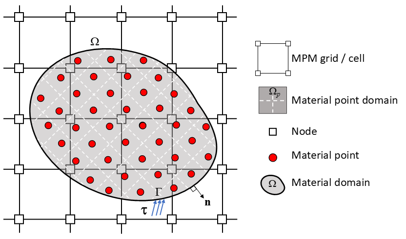
Figure 1: MPM double-discretization using material points and a computational grid.

Grid Discretization

To approximate the gradients (spatially varying fields), space is discretized by a grid (mesh), and in MPM a finite element mesh is usually used, Figure 1. This differentiates MPM from other meshfree or particle based methods such as Smooth Particle Hydrodynamics (SPH) where particle or point neighbour searching is needed. The mesh with \(n_n\) number of nodes has a basis function, or using FEM terminology, a shape function (interpolation function or kernel) \(N_i(\mathbf{x})\) associated with each node \(i\). The basis function must satisfy partition of unity for any position \(\mathbf{x}\),

(9)\[\begin{equation} \label{eq:PartUnit} \sum_{i=1}^{n_n} N_i(\mathbf{x}) = 1 \end{equation}\]

Furthermore, the position \(\mathbf{x}\) can be interpolated from the nodal coordinates \(\mathbf{x}_i\),

(10)\[\begin{equation} \label{eq:PosInter} \mathbf{x} = \sum_{i=1}^{n_n} N_i(\mathbf{x}) \mathbf{x}_i \end{equation}\]

When the position corresponds to that of a material point, \(\mathbf{x} = \mathbf{x}_p\), the following shorthand notation is used to define the interpolation weight,

(11)\[\begin{equation} \label{eq:defineWip} w_{ip} := N_i(\mathbf{x}_p) \end{equation}\]

and similarly the weight gradients (gradient of the basis function evaluated at the position of the material point),

(12)\[\begin{equation} {\nabla} w_{ip} := {\nabla} N_i(\mathbf{x}) \bigg\rvert_{\mathbf{x}=\mathbf{x}_p} = \left[\frac{\partial N_i}{\partial x_1} \ \ \frac{\partial N_i}{\partial x_2} \ \ \frac{\partial N_i}{\partial x_3}\right]^{\text{T}}_{\mathbf{x}=\mathbf{x}_p} \end{equation}\]

The virtual displacement field at the material point position \(\mathbf{t}(\mathbf{x}_p)\), for example, can be interpolated from the nodal virtual displacements \(\mathbf{t}_i\),

(13)\[\begin{equation} \label{eq:virtual_Interpolate} \mathbf{t}(\mathbf{x}_p) = \sum_{i=1}^{n_n} N_i(\mathbf{x}_p) \mathbf{t}_i :=\sum_{i=1}^{n_n} w_{ip} \mathbf{t}_i \end{equation}\]

with the spatial derivative given by,

(14)\[\begin{equation} \label{eq:Dvirtual_Interpolate} {\nabla} \mathbf{t}(\mathbf{x}_p) = \sum_{i=1}^{n_n} \left( {\nabla} N_i (\mathbf{x}) \bigg \rvert_{\mathbf{x}=\mathbf{x}_p} \mathbf{t}_i \right) := \sum_{i=1}^{n_n} {\nabla} w_{ip} \mathbf{t}_i \end{equation}\]

Similarly the acceleration field can be written as,

(15)\[\begin{equation} \label{eq:Acc_Interpolate} \mathbf{a}(\mathbf{x}_p,t) = \sum_{i=1}^{n_n} N_i(\mathbf{x}_p) \mathbf{a}_i := \sum_{i=1}^{n_n} w_{ip} \mathbf{a}_i \end{equation}\]

where \(\mathbf{a}_i\) is the nodal acceleration. Substituting Equation (13) to Equation (15) into Equation (8) leads to,

(16)\[\begin{equation} \label{eq:momWeak3} \sum_{i=1}^{n_n} \mathbf{t}_i \cdot \sum_{j=1}^{n_n} \sum_{p=1}^{n_p} m_p w_{ip} w_{jp} \mathbf{a}_j = - \sum_{i=1}^{n_n} \mathbf{t}_i \cdot \sum_{p=1}^{n_p} m_p \pmb{\sigma}_{p}^s \cdot {\nabla} w_{ip} + \sum_{i=1}^{n_n} \mathbf{t}_i \cdot \sum_{p=1}^{n_p} m_p \mathbf{b}_p w_{ip} \end{equation}\]

where \(\pmb{\sigma}_{p}^s\) = \(\pmb{\sigma}^s(\mathbf{x}_p)\) and \(\mathbf{b}_p = \mathbf{b}(\mathbf{x}_p)\) are the specific stress and body force at the material point respectively. The virtual displacement \(\mathbf{t}\) is arbitrary except where the displacement is prescribed. However, with proper constraints invoked on the displacement, the virtual displacement can be eliminated and the weak form of the momentum equation reduces to,

(17)\[\begin{equation} \label{eq:momWeak4} \sum_{i=1}^{n_n} \sum_{j=1}^{n_n} \sum_{p=1}^{n_p} m_p w_{ip} w_{jp} \mathbf{a}_j = - \sum_{i=1}^{n_n} \sum_{p=1}^{n_p} m_p \pmb{\sigma}_{p}^s \cdot {\nabla} w_{ip} + \sum_{i=1}^{n_n} \sum_{p=1}^{n_p} m_p w_{ip} \mathbf{b}_p \end{equation}\]

And in compact form, this can be written for node \(i\),

(18)\[\begin{equation} \label{eq:momCompact1} \sum_{j=1}^{n_n} m_{ij} \mathbf{a}_j = \mathbf{f}_i^{\text{int}} + \mathbf{f}_i^{\text{ext}} \end{equation}\]

where the consistent mass matrix is given by,

(19)\[\begin{equation} \label{eq:massConsist} m_{ij} := \sum_{p=1}^{n_p} m_p w_{ip} w_{jp} \end{equation}\]

The internal force vector is given by,

(20)\[\begin{equation} \label{eq:Fint} \mathbf{f}_i^{\text{int}} := - \sum_{p=1}^{n_p} \frac{m_p}{\rho_p} \pmb{\sigma}_p \cdot {\nabla} w_{ip} = - \sum_{p=1}^{n_p} V_p \pmb{\sigma}_p \cdot {\nabla} w_{ip} \end{equation}\]

where \(V_p = \frac{m_p}{\rho_p}\) is the volume of the material point. The external force vector is given by,

(21)\[\begin{equation} \label{eq:Fext} \mathbf{f}_i^{\text{ext}} := \sum_{p=1}^{n_p} w_{ip} \left(m_p \mathbf{b}_p + \mathbf{f}_p^\text{app} \right) \end{equation}\]

where \(\mathbf{f}_p^\text{app}\) is any externally applied force due to traction at the material point. The nodal acceleration is calculated by solving the system of linear equations, Equation (18). However, in MPM it is customary to replace the consistent mass matrix \(m_{ij}\) with the diagonal “lumped” mass matrix \(m_i\),

(22)\[\begin{equation} \label{eq:Mlumped} m_i := \sum_{j=1}^{n_n} m_{ij} = \sum_{p=1}^{n_p} m_p w_{ip} \end{equation}\]

The momentum Equation (18) then becomes a system of uncoupled equations,

(23)\[\begin{equation} \label{eq:momCompact2} m_{i} \mathbf{a}_i = \mathbf{f}_i^{\text{ext}} + \mathbf{f}_i^{\text{int}} \end{equation}\]

The Grid and Basis Function

The Grid

The background grid used in MPM can in theory be of any kind, but a Cartesian grid is usually chosen due to computational reasons and convenience. With a Cartesian grid it is straightforward to calculate the value of the basis function and its gradient as the function is defined in the global coordinate system. MPoint utilizes a Cartesian grid with equal node spacing \(h\) in all three cardinal directions.

The Basis Function

The original implementations of MPM all assumed a linear basis function (Sulsky et al. (1993a, 1993b, 1994, 1995) amongst many others). However, the linear functions are not ideal due to the nodal mass which can approach zero, while the internal force (based on the constant gradient) would have a finite value. The linear functions are also known for what is called the “grid-crossing instability” as described by De Vaucorbeil et al. (2020) and Steffen et al. (2010), for example. For this reason, MPoint uses a quadratic B-spline basis function.

The use of B-splines was first introduced by Steffen et al. (2008a, 2008b, 2009) to reduce the grid-crossing errors. For quadratic B-splines, the one-dimensional basis function is given by,

(24)\[\begin{split}\begin{equation} N_i^\text{1D} \left( r \right)= \begin{cases} \frac{3}{4} - |r|^2 & 0 \le |r| < \frac{1}{2} \\ \frac{1}{2} \left(\frac{3}{2} - |r|\right)^2 & \frac{1}{2} \le |r| < \frac{3}{2} \\ 0 & \frac{3}{2} \le |r| \end{cases} \end{equation}\end{split}\]

This function is shown in Figure 2 relative to the position of the nodes, and it is clear that this construction of the B-splines guarantees that the peak of the basis functions is centred at the grid nodes when equally spaced. Furthermore, the stencil (footprint) of the basis function spans \(\pm1.5h\), or a total of \(3h\), where \(h\) is the node spacing. In Figure 2 the basis function of node 3, for example, spans from (\(r - \tfrac{3}{2}h\)) to (\(r + \tfrac{3}{2}h\)). Information is projected between node 3 and all material points within this range. The gradient of the basis function is shown in Figure 3 and given by,

(25)\[\begin{split}\begin{equation} \nabla N_i^\text{1D} \left( r \right)= \begin{cases} -2r & 0 \le |r| < \frac{1}{2} \\ \left(|r| - \frac{3}{2}\right) \text{sign}(r) & \frac{1}{2} \le |r| < \frac{3}{2} \\ 0 & \frac{3}{2} \le |r| \end{cases} \end{equation}\end{split}\]

The three-dimensional basis function is the product of the one-dimensional function in each of the principal directions (\(x_1,x_2,x_3\)),

(26)\[\begin{equation} \label{eq:NNN} N_i\left(\mathbf{x}\right) = N_i^\text{1D}\left(r_1\right) N_i^\text{1D}\left(r_2\right) N_i^\text{1D}\left(r_3\right) \end{equation}\]

where \(r_1 = \tfrac{1}{h}\left(x_{1} - x_{i1}\right)\) for example. Similarly, the gradient is calculated,

(27)\[\begin{split}\begin{equation} \label{eq:dNdNdN} \nabla N_i\left(\mathbf{x}\right) = \frac{1}{h} \begin{bmatrix} \nabla N_i^\text{1D}(r_1) N_i^\text{1D}(r_2) N_i^\text{1D}(r_3) \\ N_i^\text{1D}(r_1) \nabla N_i^\text{1D}(r_2) N_i^\text{1D}(r_3) \\ N_i^\text{1D}(r_1) N_i^\text{1D}(r_2) \nabla N_i^\text{1D}(r_3) \end{bmatrix} \end{equation}\end{split}\]

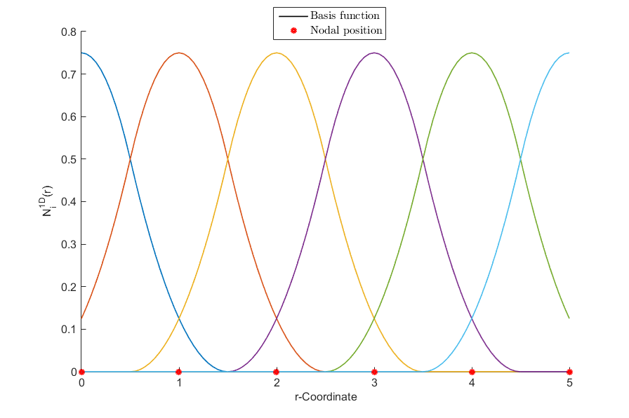
Figure 2: One-dimensional quadratic B-splines spanning six grid nodes.

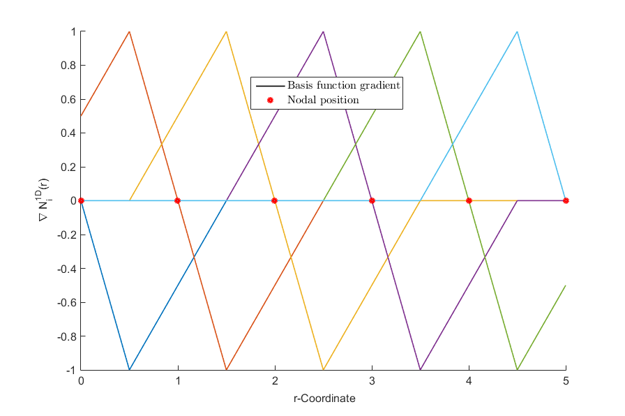
Figure 3: One-dimensional gradient of the quadratic B-splines spanning six grid nodes.

Cycling

Several time stepping schemes exist, categorised by the material point stress update. MPoint uses the update-stress-last (USL) scheme as illustrated in Figure 4, with a more detailed overview of the basic algorithm given in Table Table #tab1. For illustrative purposes, it is assumed that the basis function stencil spans only a single grid cell, i.e., assuming linear basis functions. However the principles and sreps equally apply to all types of basis functions, including the quadratic B-splines used in MPAC.

In general, four phases can be identified: (1) the material point to grid (P2G) projection, (2) the update or evolution of the grid, (3) the grid to material point (G2P) projection, and (4) the time or step increment where the superscript \(n\) is used to denote the discrete timesteps.

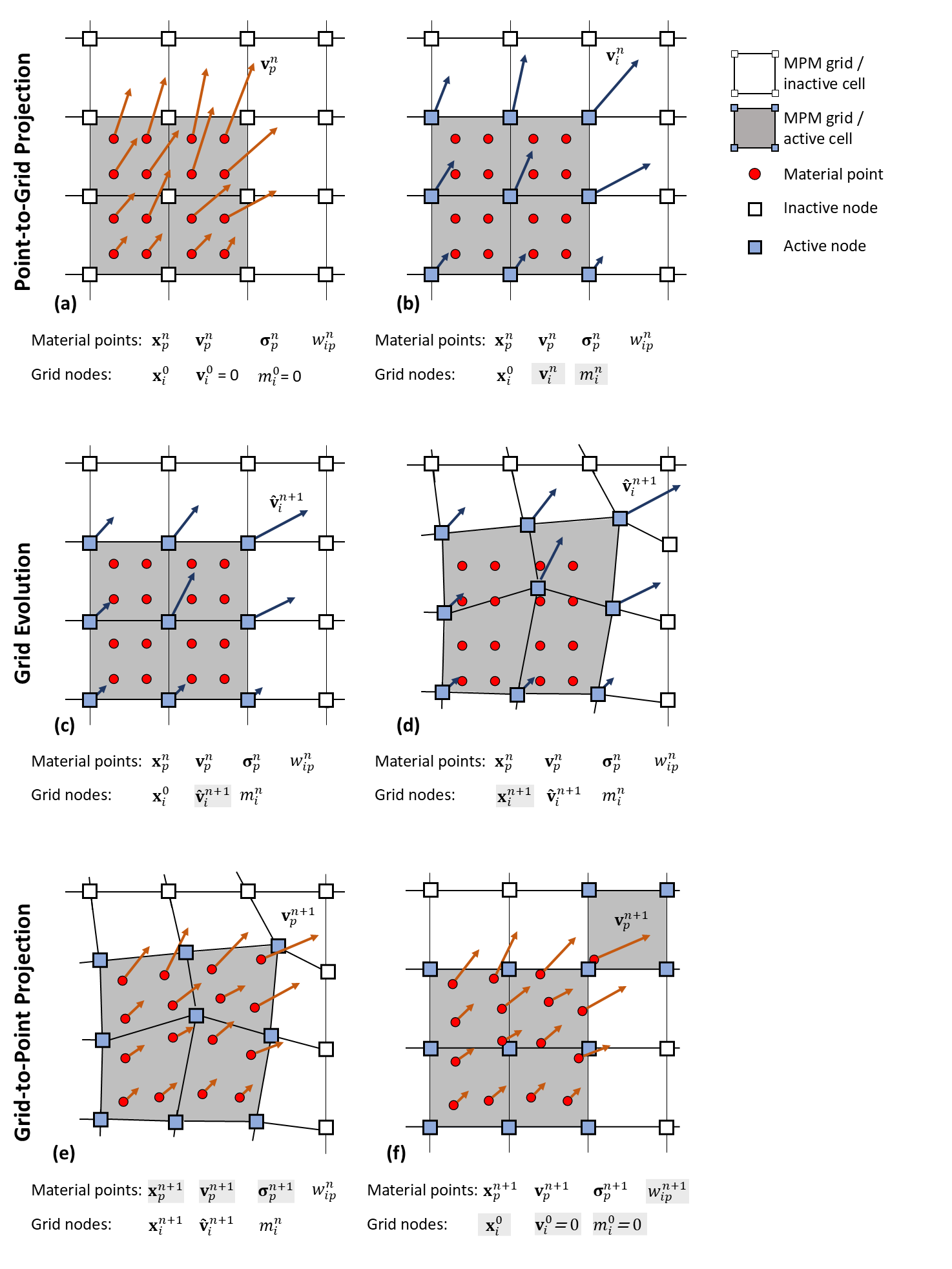
Figure 4: MPM update-stress-last (USL) cycling steps showing the update of selected state variables.

Phase 1: Point-to-Grid Projection

All state variables are recorded and carried by the material points, but the equation of motion (Equation (23)) is solved at the grid nodes. Thus, the necessary information must first be projected (mapped or interpolated) from the material points to the nodes. This phase is also referred to as the “Initialization Phase”.

The grid is initialized by setting the nodal positions \(\mathbf{x}_i^0\) and the initial nodal velocity \(\mathbf{v}_i^0 = 0\) and mass \(m_i^0=0\), Figure 4 (a). Each material point has a known position \(\mathbf{x}_p^n\) at timestep \(n\) and stores a constant mass \(m_p\) and a velocity \(\mathbf{v}_p^n\) (the momentum). Using the basis function and the position of the material point relative to the nodes, the weights \(w_{ip}^n\) can be calculated using Equation (11) and Equation (26). Note that the weight \(w_{ip}^n\) is computed at timestep \(n\) and the material point can move through the grid, thus the weight is time-dependent). The mass is projected to grid node \(i\) by summing over all the materials points within the node’s stencil (Equation (22)),

(28)\[\begin{equation} \label{eq:nodalMass} m_i^n = \sum_{p=1}^{n_p} m_p w_{ip}^n \end{equation}\]

The material point momentum \(\mathbf{p}_p^n := m_p \mathbf{v}_p^n\) is projected to the grid nodes. Since there are in general more material points than grid nodes, a weighted least-squares (with the weight equal to the material point’s mass) projection is used. The nodal momentum \(\mathbf{p}_i^n\) follows as,

(29)\[\begin{equation} \label{eq:NodalMom} \mathbf{p}_i^n := m_i^n \mathbf{v}_i^n = \sum_{p=1}^{n_p} m_p w_{ip}^n \left(\mathbf{v}_p^n + \nabla \mathbf{v}_p^{n} (\mathbf{x}_i - \mathbf{x}_p^n)\right) \end{equation}\]

where \(\nabla \mathbf{v}_p^{n}\) is the velocity gradient evaluated at the material point at the end of the previous timestep (Wallstedt and Guilkey, 2007).

Note

The velocity gradient term in Equation (29) is often omitted. However, Nakamura et al. (2023) point out that using the velocity gradient to enhance the velocity projection is fundamentally a first-order Taylor series approximation of the point’s velocity in space. In literature, this is referred to as the “Taylor transfer” (TPIC or TFLIP depending on the update of the material point velocity). The Taylor transfer is a type of affine transfer (APIC and AFLIP) and Duverger et al. (2025): found it to be “the most suitable motion integration strategy”.

Finally, the nodal velocity is obtained using,

(30)\[\begin{equation} \label{eq:NodalVel1} \mathbf{v}_i^n = \frac{\mathbf{p}_i^n }{m_i^n} \end{equation}\]

to provide the nodal velocity at the start of the time step, Figure 4 (b).

Phase 2: Grid Evolution

This phase is also referred to as the “Lagrangian Phase” due to the similarities with updated Lagrangian FEM. The internal and external nodal forces are calculated using Equation (20) and Equation (21) respectively, and used to solve for the nodal acceleration \(\mathbf{a}_i^n\) which is trivial if a lumped mass matrix is used (Equation (23)),

(31)\[\begin{equation} \label{eq:acc} \mathbf{a}_i^n = \frac{1}{m_i^n} \left( \mathbf{f}_i^{\text{ext,}n} + \mathbf{f}_i^{\text{int,}n} \right) \end{equation}\]

Using explicit central-difference integration with time increment \(\Delta t\), the nodal velocity is updated, Figure 4 (c),

(32)\[\begin{equation} \label{eq:vNodeUpdate} \mathbf{\tilde{v}}_i^{n+1} = \mathbf{v}_i^{n} + \Delta t \mathbf{a}_i^n \end{equation}\]

At this point, boundary conditions are be applied to the nodes by setting \(\mathbf{\tilde{v}}_i^{n+1} = \mathbf{v}_i^{\text{fix},n}\), where \(\mathbf{v}_i^{\text{fix},n}\) is the current zero or non-zero fixed velocity. For nodes with fixities, the acceleration is then recalculated using \(\mathbf{a}_i^n = \left(\mathbf{\tilde{v}}_i^{n+1} - \mathbf{v}_i^n\right) / \Delta t\)

Note

Note that the use of non-zero velocity fixities applied to the nodes is not very useful in MPM since the material points might move away from the nodes where the fixity is applied. It is better to use material point fixities as DISCUSSED HERE-XXXXXXXXX.

Note

The updated nodal velocity is written as \(\mathbf{\tilde{v}}_i^{n+1}\) and not \(\mathbf{{v}}_i^{n+1}\). This is to due to the grid being reset at the end of the time step and in theory the nodal velocity reset to zero. During phase 1 of the next time step (\(n+1\)) the point velocity is projected to the grid to obtain \(\mathbf{{v}}_i^{n+1}\) (Equation (30)) which is different from \(\mathbf{\tilde{v}}_i^{n+1}\).

In theory the nodal position is updated, Figure 4 (d),

(33)\[\begin{equation} \label{eq:GridPosUpdate} \mathbf{x}_i^{n+1} = \mathbf{x}_i^{n} + \Delta t \mathbf{\tilde{v}}_i^{n+1} \end{equation}\]

This update of the grid position is not explicitly performed in most MPM implementations, and the material points can be directly updated as discussed below. However, it is important to understand that in theory the grid also displaces and the material points displace with the grid as defined by the basis function. In FEM terms, if local element coordinates were defined, the material points would remain at the same local coordinates until the grid is reset right at the end of the time step, i.e., the weights \(w_{ip}\) remain constant during this phase.

Phase 3: Grid-to-Point Projection

With the grid updated, the changes are projected back to the material points where the velocity, position, strain, stress, deformation gradient, volume and density are updated, Figure 4 (e).

Velocity Update

There are two approaches to update the material point velocity, namely “fluid-implicit-particle” (FLIP) and “particle-in-cell” (PIC). In FLIP, only the change in grid velocity \(\left( \mathbf{\tilde{v}}_i^{n+1} - \mathbf{v}_i^{n} \right)\) is interpolated to update the material point velocity,

(34)\[\begin{split}\begin{align} \label{eq:FLIPvel} \mathbf{v}_p^{n+1} &= \mathbf{v}_p^{n} + \sum_{i=1}^{n_n} w_{ip}^n \left( \mathbf{\tilde{v}}_i^{n+1} - \mathbf{v}_i^{n} \right) \nonumber \\ &= \mathbf{v}_p^{n} + \Delta t \sum_{i=1}^{n_n} w_{ip}^n \mathbf{a}_i^{n} \end{align}\end{split}\]

In PIC, the updated grid velocity \(\mathbf{\tilde{v}}_i^{n+1}\) is used to set the material point velocity,

(35)\[\begin{equation} \label{eq:PICvel} \mathbf{v}_p^{n+1} = \sum_{i=1}^{n_n} w_{ip}^n \mathbf{\tilde{v}}_i^{n+1} \end{equation}\]

A weighted combination of FLIP and PIC update using the scalar \(\alpha\) is available in MPoint,

(36)\[\begin{equation} \label{eq:FLIPPICvel} \mathbf{v}_p^{n+1} = \sum_{i=1}^{n_n} w_{ip}^n \mathbf{\tilde{v}}_i^{n+1} + \alpha \left( \mathbf{v}_p^{n} - \sum_{i=1}^{n_n} w_{ip}^n \mathbf{v}_i^n \right) \end{equation}\]

When \(\alpha = 0\), PIC transfer is obtained and when \(\alpha = 1\), FLIP transfer is obtained. Setting \(0 < \alpha < 1\) provides a weighted FLIP-PIC transfer. In MPoint, \(\alpha = 1\) is used by default.

Note

For a more in-depth discussion on FLIP and PIC transfers and PIC damping, see the description here.

Position Update

The position of the material points is updated using the nodal acceleration and the new nodal velocity \(\mathbf{\tilde{v}}_i^{n+1}\) in a second-order scheme (Nairn and Hammerquist (2021)),

(37)\[\begin{equation} \label{eq:posUpdate1} \mathbf{x}_p^{n+1} = \mathbf{x}_p^{n} + \Delta t \sum_{i=1}^{n_n} w_{ip}^n \mathbf{\tilde{v}}_i^{n+1} + \left(\Delta t\right)^2 \sum_{i=1}^{n_n} w_{ip}^n \mathbf{a}_i^{n} \end{equation}\]

Velocity Gradient and Deformation Gradient Update

The velocity gradient \(\nabla \mathbf{v(\mathbf{x})}\) is calculated at the material points based on the updated nodal velocity and Equation (14),

(38)\[\begin{equation} \label{eq:velGrad} \nabla \mathbf{v}_p^{n+1} := \nabla \mathbf{v(\mathbf{x})} \rvert_{\mathbf{x}=\mathbf{x}_p}^{n+1} = \sum_{i=1}^{n_n} \nabla w_{ip}^n \mathbf{\tilde{v}}_i^{n+1} \end{equation}\]

The deformation gradient \(\mathbf{F}_p^n\) is updated at the material points,

(39)\[\begin{equation} \label{eq:defGrad} \mathbf{F}_p^{n+1} = \left(\mathbf{I} + \Delta t \ {\nabla} \mathbf{v}_p^{n+1} \right) \mathbf{F}_p^n \end{equation}\]

where \(\mathbf{I}\) is the identity matrix.

Volume and Density Update

The volume \(V_p\) of the material point is updated using the determinant of the deformation gradient \(J\),

(40)\[\begin{equation} \label{eq:volumeUpdate} V_p^{n+1} = J_p^{n+1} V_p^0 \quad \text{where} \quad J_p^{n+1} := \det (\mathbf{F}_p^{n+1}) \end{equation}\]

where \(V_p^0\) is the point’s initial volume. Lastly the material point’s density is updated,

(41)\[\begin{equation} \label{eq:densityUpdate} \rho_p^{n+1}= \frac{\rho_p^0}{J_p^{n+1}} \end{equation}\]

where \(\rho_p^0\) is the point’s initial density.

Strain and Stress Update

The increment in strain (based on Equation (3)) at the material point then follows from,

(42)\[\begin{equation} \label{eq:strain2} \Delta \pmb{\varepsilon}_p = \frac{\Delta t}{2} \left[\nabla \mathbf{v}_p^{n+1} + \left(\nabla \mathbf{v}_p^{n+1} \right)^\text{T}\right] \end{equation}\]

and the strain is updated according to,

(43)\[\begin{equation} \label{eq:strain3} \pmb{\varepsilon}_p^{n+1} = \pmb{\varepsilon}_p^{n} + \Delta \pmb{\varepsilon}_p \end{equation}\]

An appropriate constitutive model is then used to calculate the increment in stress (\(\Delta \pmb{\varepsilon}_p \rightarrow \Delta \pmb{\sigma}_p\)) at each material point which is used to update the stress,

(44)\[\begin{equation} \label{eq:stress1} \pmb{\sigma}_p^{n+1} = \pmb{\sigma}_p^{n} + \Delta \pmb{\sigma}_p \end{equation}\]

Note that the material points do not all have to make use of the same constitutive model, a different constitutive model can be assigned to each point or to (spatially) grouped points for example.

Phase 4: Time Increment

With all of the state variables fully updated at the material points, the grid is reset (nodal positions restored to \(\mathbf{x}_i^0\)) as shown in Figure 4 (f). Although the nodal positions are in practise not explicitly updated, in theory the resetting of the grid results in the movement of the points relative to the grid. Also, the grid does not have to be reset to the same configuration, but can at this stage also be updated and refined for example, or alternatively a completely new grid can be introduced. However, whether the grid is reset, modified or a new grid introduced, if the position of the material points changed relative to the nodal positions, new weights \(w_{ip}^{n+1}\) and gradients \(\nabla w_{ip}^{n+1}\) should be computed and the grid mass and velocity (momentum) set to zero.

Timestep

The size of the critical (stable) timestep \(\Delta t_{\text{crit}}\) is calculated using the Courant-Friederichs-Lewy (CFL) condition,

(45)\[\begin{equation} \label{eq:CFL} \Delta t_{\text{crit}} = \frac{h}{\max(c_p + \left\| \mathbf{v}_p\right\|)} \end{equation}\]

where \(h\) is the grid node spacing, \(\mathbf{v}_p\) is the speed of the material point and \(c_p\) is the speed of sound in the material,

(46)\[\begin{equation} \label{eq:SpeedSound} c_p = \sqrt{\frac{K+\frac{4}{3}G}{\rho}} \end{equation}\]

where \(K = E/(3(1+\nu))\) and \(G = E/(2(1+\nu))\) are the material’s bulk and shear stiffness respectively, \(E\) and \(\nu\) the Young’s modulus and Poisson’s ratio and \(\rho\) the density.

Volumetric Locking

Similar to mesh-based methods, such as the finite element method, the material point method (MPM) is susceptible to volumetric locking. In MPM the material points, which act as integration points, are allowed to move through the background grid. This can reduce the accuracy of integration if there is not a sufficient number of points per background cell. To overcome this, the number of points is usually increased, resulting in more points per cell then the number of Gauss integration points for an identical FEM element. The locking is mainly due to excessive constraints placed on the cell’s deformation by the relatively large number of integration points. This, combined with lower-order basis functions (interpolation or shape functions), results in volumetric locking when modelling near-incompressible materials (Coombs et al., 2018). Using a higher-order basis function (such as the quadratic B-splines used in MPoint) can reduce the locking effects, but this is not enough to reduce locking to acceptable levels (Telikicherla and Moutsanidis, 2022:). Furthermore, without strict control over the number of material points per cell as they move through the grid, reduced integration often used in FEM, is not an option in MPM.

The velocity gradient \(\nabla \mathbf{v}_p\) at a material point can be decomposed into a dilational (volumetric) component \(\nabla \mathbf{v}_p^\mathrm{dil}\) and a deviatoric component \(\nabla \mathbf{v}_p^\mathrm{dev}\),

(47)\[\begin{equation} \label{eq:lock1} \nabla \mathbf{v}_p = \nabla \mathbf{v}_p^\mathrm{dil} + \nabla \mathbf{v}_p^\mathrm{dev} \end{equation}\]

where

(48)\[\begin{equation} \label{eq:lock2} \nabla \mathbf{v}_p^\mathrm{dil} = \frac{1}{d}\left(\nabla \cdot \mathbf{v}_p\right) \mathbf{I} = \frac{1}{d} \mathrm{tr} \left(\nabla \mathbf{v}_p\right) \mathbf{I} \end{equation}\]

(49)\[\begin{equation} \label{eq:lock3} \nabla \mathbf{v}_p^\mathrm{dev} = \nabla \mathbf{v}_p - \nabla \mathbf{v}_p^\mathrm{dil} \end{equation}\]

and \(d\) is the model dimension (\(d=2\) for two-dimensional and \(d=3\) for three-dimensional), and \(\mathbf{I}\) is the identity matrix. To overcome locking, the dilational component \(\nabla \mathbf{v}_p^\mathrm{dil}\) is replaced by an improved dilational component \(\overline{\nabla \mathbf{v}}_p^\mathrm{dil}\), while the deviatoric part remains unchanged. Suppose that such an improved dilational component can be found, then Equation (47) can be written as,

(50)\[\begin{equation} \label{eq:lock4} \overline{\nabla \mathbf{v}}_p = \overline{\nabla \mathbf{v}}_p^\mathrm{dil} + \nabla \mathbf{v}_p^\mathrm{dev} \end{equation}\]

where \(\overline{\nabla \mathbf{v}}_p\) is the improved total velocity gradient. Using Equation (49), Equation (50) can be written as,

(51)\[\begin{equation} \label{eq:lock5} \overline{\nabla \mathbf{v}}_p =\nabla \mathbf{v}_p + \overline{\nabla \mathbf{v}}_p^\mathrm{dil} - \nabla \mathbf{v}_p^\mathrm{dil} \end{equation}\]

and using Equation (48), it becomes,

(52)\[\begin{equation} \label{eq:lock6} \overline{\nabla \mathbf{v}}_p =\nabla \mathbf{v}_p + \frac{1}{d}\left(\overline{\nabla \cdot \mathbf{v}}_p - \nabla \cdot \mathbf{v}_p\right) \mathbf{I} \end{equation}\]

There are various ways to find an improved dilational component of the velocity gradient, and in MPoint, the cell-averaged value is used,

(53)\[\begin{equation} \label{eq:lock7} \overline{\nabla \cdot \mathbf{v}}_p = \left(\nabla \cdot \mathbf{v} \right)_c := \frac{{\sum_{p=1}^{n_{pc}} \left(\nabla \cdot \mathbf{v}_p \right) V_p}}{{\sum_{p=1}^{n_{pc}} V_p}} \end{equation}\]

where \(\left(\nabla \cdot \mathbf{v} \right)_c\) is the cell-averaged value, \(n_{pc}\) is the number of material points in the background cell, \(\nabla \cdot \mathbf{v}_p\) is the dilational component of the velocity gradient at the material point, and \(V_p\) is the material point volume.

After calculating the velocity gradient at the material points, the dilational component from all material points within a background cell is averaged using the material point volume as weight, Equation (53). This cell-centered value is then used to calculate an improved velocity gradient at each of the material points within the cell, Equation (52).

Note

The improved velocity gradient (steps 7.1 and 8.1 in Table Table #tab1) is used to compute the material point strain update, followed by the stress update (steps 8.2 and 8.3). The deformation gradient, volume, and density are still updated with the velocity gradient as calculated before (steps 6.1 to 6.3).

Basic Cycling Overview

An overview of the cycling steps is shown in Figure 5. Note that steps 7.1 and 8.1 are executed only if volumetric locking is adjusted. Step 2 deals with material point fixities, and step 9 with splitting. These are discussed here XXXXXX and here XXXXX.

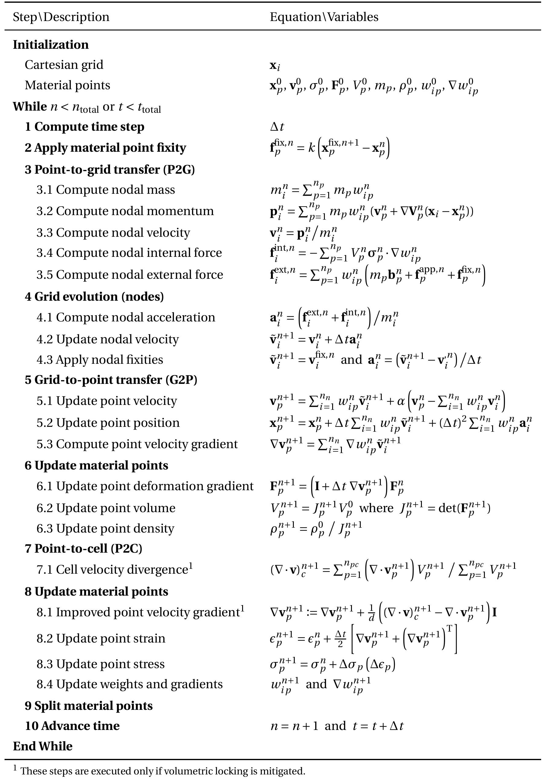
Figure 5: Overview of the MPoint cycling steps (without FLAC coupling).

FLIP-PIC Velocity Update

Due to the double discretisation in MPM using material points and grid nodes, momentum (or velocity and mass), need to be projected from material points to grid nodes (point-to-grid) and vice versa (grid-to-point). Both projections happen once per timestep as discussed in the cycling steps.

The projection of momentum from material points to grid nodes is given by (Equation (29) repeated here for convenience),

(54)\[\begin{equation} \label{eq:NodalMomRepeat} \mathbf{p}_i^n := m_i^n \mathbf{v}_i^n = \sum_{p=1}^{n_p} m_p w_{ip}^n \left(\mathbf{v}_p^n + \nabla \mathbf{v}_p^{n} (\mathbf{x}_i - \mathbf{x}_p^n)\right) \end{equation}\]

Since there are generally more material points than active grid nodes, the total number of degrees-of-freedom of the materials points is larger than that of the grid. Due to this, some material point velocity modes are not captured by the grid nodes (does not reflect on the grid nodes). The lost modes are often referred to as “null-modes” (Jiang et al., 2016).

For the projection of velocity from the grid nodes to the material points, two general strategies are available as mentioned here, namely FLIP and PIC. Alternatively a weighted combination of the two strategies, called FLIP-PIC, can be used. In FLIP, the transfer is as follow (Equation (34)),

(55)\[\begin{equation} \label{eq:FLIPvel2} \mathbf{v}_p^{n+1} = \mathbf{v}_p^{n} + \sum_{i=1}^{n_n} w_{ip}^n \left( \mathbf{\tilde{v}}_i^{n+1} - \mathbf{v}_i^{n} \right) \end{equation}\]

and in PIC, the transfer is given by (Equation (35)),

(56)\[\begin{equation} \label{eq:PICvel2} \mathbf{v}_p^{n+1} = \sum_{i=1}^{n_n} w_{ip}^n \mathbf{\tilde{v}}_i^{n+1} \end{equation}\]

The first observation is that in FLIP, only the change in nodal velocity is projected to a material point where it is used to update or increment its velocity. On the other hand, in PIC, the updated nodal velocity is projected to a material point where it is used to set its velocity (not incremented).

The difference in FLIP and PIC update is related to the effects of the null-modes where some material point velocity modes do not reflect on the grid. After solving the equation of motion, the grid velocity is updated, and if this updated velocity is projected to the material points using PIC transfer, the null-modes are filtered out. In other words, the material point velocity modes not seen on the grid, are filtered out and the material point modes are overwritten by that of the lower resolution grid (Fu et al., 2017). This is the reason why PIC transfer is generally associated with high levels of energy dissipation and little noise.

On the other hand, when FLIP transfer is used, only the change in grid velocity is projected to the material point where it is used to increment its velocity, i.e, the material point velocity is not completely overwritten with the lower resolution velocity from the grid. Thus, the null velocity modes are not lost and the excessive dissipation of PIC avoided. However, the material point velocity modes not seen by the grid persists and do not receive the appropriate constitutive response (velocity gradients and thus strain and stress increments are based on the node velocity) and the errors can accumulate and affect the solution. Thus, FLIP transfer is less dissipative, but has more artificial noise.

A weighted combination of FLIP and PIC velocity update (Equation (36)) was first introduced by Stomakhin et al. (2013),

(57)\[\begin{equation} \label{eq:FLIPPICvel_APP} \mathbf{v}_p^{n+1} = \sum_{i=1}^{n_n} w_{ip}^n \mathbf{\tilde{v}}_i^{n+1} + \alpha \left( \mathbf{v}_p^{n} - \sum_{i=1}^{n_n} w_{ip}^n \mathbf{v}_i^n \right) \end{equation}\]

When \(\alpha = 0\) the PIC transfer is obtained and when \(\alpha = 1\) the FLIP transfer is obtained (the default in MPoint). Setting \(0 < \alpha < 1\) provides a weighted FLIP-PIC transfer. Nairn (2015) rewrote Equation (57) as follow,

(58)\[\begin{equation} \label{eq:FLIPPICvel_Nairn} \mathbf{v}_p^{n+1} = \mathbf{v}_p^{n} + \left( \sum_{i=1}^{n_n} w_{ip}^n \mathbf{a}_i^n -\beta\left( \mathbf{v}_p^{n} -\sum_{i=1}^{n_n} w_{ip}^n \mathbf{v}_i^n \right) \right) \Delta t \end{equation}\]

where

(59)\[\begin{equation} \label{eq:Beta} \beta = \frac{(1-\alpha)}{\Delta t} \end{equation}\]

is a “PIC damping coefficient”.

Nairn (2015) suggests that \(\beta\) (and indirectly \(\alpha\)) acts as a damping coefficient, where Equation (58) has the standard form of damping where the acceleration is reduced by a term proportional to velocity. The damping term consists of the difference between two velocities, namely the point velocity \(\mathbf{v}_p^n\) and the grid node velocity \(\mathbf{v}_i^n\) projected to the material point. In a ‘well-behaved’ simulation, the difference between these two velocities would be small, and the update would be close to that of pure FLIP. However, when there is a difference between these two velocities, due to null modes for example where material point velocity modes are not reflected on the grid, the PIC component of the transfer dampens such noise.

Comparison with the Finite Element Method

The governing equations in their strong form (Equation (1) and Equation (2)) are identical to that used in FEM. The form of the discrete momentum equation (Equation (18) or Equation (23) depending on the use of a consistent or lumped mass matrix) is identical to that of FEM, however, the calculation of the individual terms are different.

In FEM, the internal force vector is given by,

(60)\[\begin{equation} f_{i}^{\text{int}} = - \int_{\Omega} \pmb{\sigma} \cdot {\nabla} Q_i \text{d}\Omega \end{equation}\]

where \(Q_i\) are the element shape functions. The integral is evaluated using numerical integration or numerical quadrature rules. Quadrature (integration) points are defined at fixed positions within the element, each with a weight \(w_q\). The calculation of the internal force then reduces to summation over the integration points \(n_q\),

(61)\[\begin{equation} f_{i}^{\text{int}} = - \sum_{q=1}^{n_q} w_q \pmb{\sigma}_q \cdot {\nabla} Q_i(\mathbf{x}) \rvert_{\mathbf{x}=\mathbf{x}_q} \ d \Omega \end{equation}\]

Comparing this to Equation (20), reveals that MPM is identical to FEM in this regard if the material points are considered integration points, and their integration weight is set equal to their volume (\(w_q = V_p\)). The same principle applies to the mass matrix and the external force vector.

References

Coombs, W.M., T.J. Charlton, M. Cortis, and C.E. Augarde. “Overcoming volumetric locking in material point methods”, Computer Methods in Applied Mechanics and Engineering 333, 1–21 (2018).

De Vaucorbeil, A., V.P. Nguyen, S. Sinaie, and J.Y. Wu. “Material point method after 25 years: Theory, implementation, and applications”, Advances in Applied Mechanics 53, 185–398 (2020).

Duverger, S., J. Duriez, P. Philippe, and S. Bonelli. “Critical Comparison of Motion Integration Strategies and Discretization Choices in the Material Point Method”, Archives of Computational Methods in Engineering 32(3), 1369–1397 (2025).

Fu, C., Q. Guo, T. Gast, C. Jiang, and J. Teran. “A polynomial particle-in-cell method”, ACM Transactions on Graphics 36(6) (2017).

Jiang, C., C. Schroeder, and J. Teran. “An angular momentum conserving affine-particle-in-cell method”, Journal of Computational Physics 338, 137–164 (2017).

Nairn, J.A. “Numerical simulation of orthogonal cutting using the material point method”, Engineering Fracture Mechanics 149, 262–275 (2015).

Nairn, J.A. and C.C. Hammerquist. “Material point method simulations using an approximate full mass matrix inverse”, Computer Methods in Applied Mechanics and Engineering 377, 1–21 (2021).

Nakamura, K., S. Matsumura, and T. Mizutani. “Taylor particle-in-cell transfer and kernel correction for material point method”, Computer Methods in Applied Mechanics and Engineering 403, 115720 (2023).

Steffen, M., P.C. Wallstedt, J.E. Guilkey, R.M. Kirby, and M. Berzins. “Examination and analysis of implementation choices within the Material Point Method (MPM)”, CMES - Computer Modeling in Engineering and Sciences 31(2), 107–127 (2008).

Steffen, M., R.M. Kirby, and M. Berzins. “Analysis and reduction of quadrature errors in the material point method (MPM)”, International Journal for Numerical Methods in Engineering 76(6), 922–948 (2008).

Steffen, M. “Analysis-guided improvements of the material point method”, Phd, The University of Utah (2009).

Steffen, M., R.M. Kirby, and M. Berzins. “Decoupling and balancing of space and time errors in the material point method (MPM)”, International Journal for Numerical Methods in Engineering 82(10), 1207–1243 (2010).

Stomakhin, A., C. Schroeder, L. Chai, J. Teran, and A. Selle. “A material point method for snow simulation”, ACM Transactions on Graphics 32(4) (2013).

Sulsky, D., and H. Schreyer. “A particle-in-cell method as a natural impact algorithm”, Advanced Computational Methods for Material Modeling, ASME AMD-Vol. 1 (1993a).

Sulsky, D., and H. Schreyer. “A particle method with large rotations applied to the penetration of history-dependent materials”, Advances in Numerical Simulation Techniques for Penetration and Perforation of Solids, ASME 171 (1993b).

Sulsky, D., Z. Chen, and H. Schreyer. “A particle method for history-dependent materials”, Comput. Methods Appl. Mech. Engrg. 118, 179–196 (1994).

Sulsky, D.L., S.L. Zhou, and H. Schreyer. “Application of a particle-in-cell method to solid mechanics”, Computer Physics Communications 87, 236–252 (1995).

Telikicherla, R.M. and G. Moutsanidis. “Treatment of near-incompressibility and volumetric locking in higher order material point methods”, Computer Methods in Applied Mechanics and Engineering 395(2022).

Wallstedt, P.C., and J.E. Guilkey. “Improved velocity projection for the material point method”, CMES - Computer Modeling in Engineering and Sciences 19(3), 223–232 (2007).