Cyclic Undrained DSS Tests with P2PSand Model (FLAC2D)

Verification Problem

The project file for this example may be viewed/run in FLAC2D.[1] The main data file used is shown at the end of this example.

How To Read and Use Examples

One-zone numerical tests of undrained cyclic direct simple shear (DSS) loading responses are performed. All these tests are starting from an initial effective vertical stress (\(\sigma^{\prime}_{v0}\)) along z-axis at 100 kPa (around 1 atm), \(K_0=0.5\), and zero initial static shear stresses.

All parameters are with the default parameters except the initial relative densities are different. Pore-pressure in the zone is allowed for building-up. The out-of-plane (alone y-axis) strains are restricted. The degrees-of freedom at the zone top are attached so that all grid points at the top have the same displacements to satisfy the DSS conditions. The gridpoints at the zone top are velocity-controlled. Once the shear stress (\(\tau\)) amplitude reaches a certain value (\(CSR \times \sigma^{\prime}_{v0}\)), the velocities of gridpoints at the zone top will be reverted. In this example, the parameter study is performed by a Python-based master file.

The numerical results of undrained cyclic DSS loading responses with the relative density at \(D_r\) = 0.3, 0.5 and 0.7, are illustrated in Figure 1, 2 and 3, to represent relative loose, median dense and dense sands, respectively. In each of the figures, the top sub-figure is plotting \(\sigma^{\prime}_v/\sigma^{\prime}_{v0}\) versus \(\tau_{xz}/\sigma^{\prime}_{v0}\), the center sub-figure is plotting \(\sigma^{\prime}_v/\sigma^{\prime}_{v0}\) versus \(\gamma\), and the bottom sub-figure is plotting \(R_u\) versus \(\gamma\). All illustrated responses reach about \(\gamma = 3\%\) (S.A.) shear strain with the fitted CSR values at approximately 15 cycles. The shear stress - shear strain responses illustrate shear strain progresses even after the excess pore pressure ratio (\(R_u\)) reaches 99%.

For relatively loose sands as shown in Figure 1, the shear strain increases to a very small value at the first several cycles. After dilatancy surface has been hit, the shear strain dramatically increases to around 3% \(\sigma^{\prime}_v\) is close to 0, and \(R_u\) is close to 1, merely after a couple of extra cycles. For relative dense sands as shown in Figure 3, the shear strain increases approximately in each cycle, rather than just the last few cycles as seen in the relatively loose sands. The median dense sands (Figure 2) presents intermediate behaviors as expected.

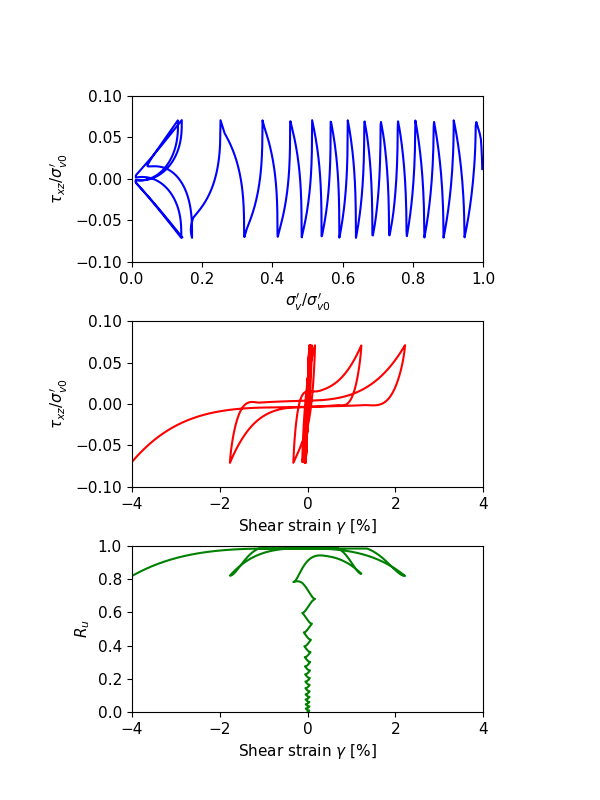
Figure 1: Undrained cyclic DSS loading response for \(D_r\) = 0.3.

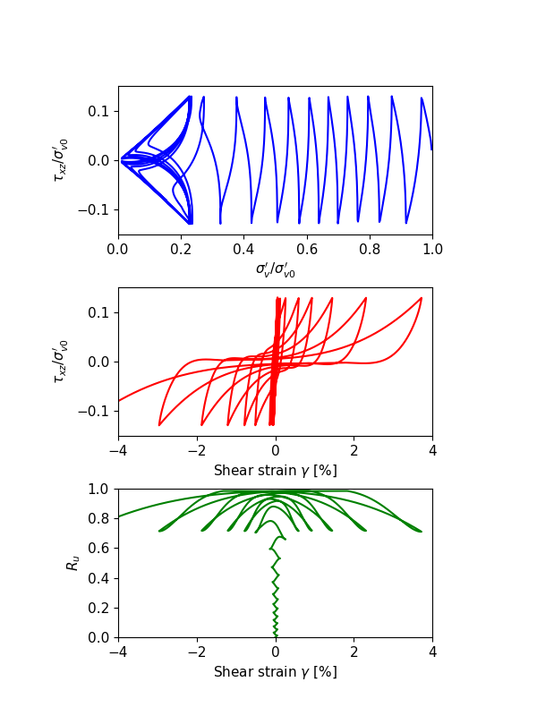
Figure 2: Undrained cyclic DSS loading response for \(D_r\) = 0.5.

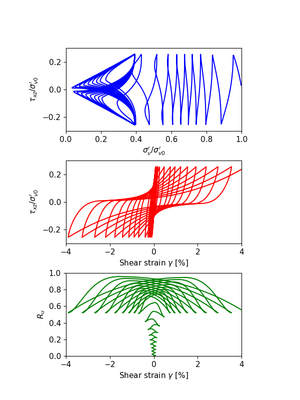
Figure 3: Undrained cyclic DSS loading response for \(D_r\) = 0.7.

The trend of the simulated results for sands from loose to dense state is consistent to the general observations: At the same other conditions, a denser sand have a higher CSR value. As the relative density is increasing, the deformation mode is transferring from liquefaction flow to cyclic mobility. Stress-strain loops for loose sands contain flat segments, a phenomenon term as “neutral phase”, where little or small shear stiffness develops during deformation; stress-strain loops for dense sands have no-zero sloping segments indicating significantly higher shear resistance.

The results by P2PSand model are compared with the empirical curves by Youd et al (2001) and Idriss and Bounlanger (2008) in Figure 4. The relation of \((N_1)_{60} = 46D_r^2\) is used.

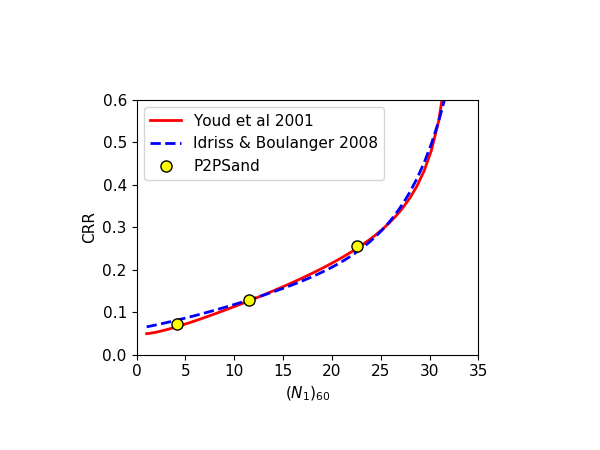
Figure 4: CRR vs. \((N_1)_{60}\).

Data File

CyclicUndrainedDirectSimpleShear.dat

model large-strain off
model configure dynamic

program call 'input'
[input_parameters]
;
zone create quadrilateral size (1,1)
; assign constitutive model
zone cmodel assign p2psand

;;; initial conditions
zone initialize stress-xx [-Sv0*K0]
zone initialize stress-zz [-Sv0*K0]
zone initialize stress-yy [-Sv0]

;;; material properties
zone property density [rho_d] pressure-reference [Patm] factor-cut 0.01
;;; input equivalent relative-density-initial corresponding to field condition
zone property relative-density-initial [dr0] 
;;; or directly input (N1)60 in field condition
;zone property n-1-60 [46.0*dr0*dr0]
;;; initial stresses should be input as properties when p2psand model
;;; is first assigned
fish operator ini_stress(z, modelname)
    if zone.model(z) == modelname then 
        zone.prop(z,'stress-initial') = zone.stress.effective(z)
    endif
end
[ini_stress(::zone.list, 'p2psand')]

;;; assign water constitutive model
model configure fluid-flow
model fluid active off
zone fluid property pore-pressure-generation on
zone fluid property effective-cutoff -1e20
zone fluid property mobility-coefficient [poro]
zone fluid property fluid-density [dw] fluid-modulus [Kw]

;;; boundary conditions
zone gridpoint fix velocity range position-y 0
zone attach gridpointid 3 to-gridpointid 4 snap off

;;; apply conditions
zone face apply stress-yy [-Sv0] range position-y 1.0

model dynamic time-total 0
;
[global zptr1 = zone.find(1)]
fish define rup
    local s = zone.stress.effective(zptr1)
    rup = (p0 + (s->xx+s->yy)/2.0)/p0
end
;
zone dynamic damping rayleigh 0.002 1
model dynamic timestep fix 4.0e-5
;
history interval 25
model history dynamic time-total
zone history displacement-x gridpointid 4
zone history stress-xy zoneid 1
zone history stress-effective-yy zoneid 1
fish history [rup]
;
zone gridpoint fix velocity-x [rate] range position-y 1
;
[global gptr1 = gp.near(1,1)]
fish define toThisShearStrain
    return math.abs(gp.disp(gptr1)->x) >= ssv
end
;
[global top = gp.list(gp.pos(::gp.list)->y==1)]
fish define cyclic
    local xy = zone.stress(zptr1)->xy
    if xy >  csr*Sv0 then gp.vel(::top)->x = -rate
    if xy < -csr*Sv0 then gp.vel(::top)->x =  rate
end
;
model solve dynamic time-total 2000 ...
    fish-halt [toThisShearStrain] ...
    fish-call -20 [cyclic]
    
;   
history export '1' '2' '3' '4' '5' file [txtfile] truncate
model save [savefile]

Endnote

[1]

This example is listed under the present document title in the i Examples dialog (use the menu command Help -> Examples… to access).