Examples • Verification Problems

Uniaxial Compressive Strength of a Jointed Material Sample (3DEC)

Problem Statement

Note

The project file for this example is available to be viewed/run in 3DEC.[1] The main data files used are shown at the end of this example. The remaining data files can be found in the project.

The uniaxial compressive strength of a cylindrical sample of material is evaluated numerically using the ubiquitous-joint model. This model takes into consideration a direction of weakness (ubiquitous-joint) in a Mohr-Coulomb material on which shear failure can be initiated. The compressive strength of the sample is a function of the material and joint properties, as well as the angle, \(\beta\), formed by the direction of the compressive stress and its projection onto the plane of weakness (see Figure 1).

In this example, the sample is selected as a cylinder with radius, \(a\), and height, \(b\), such that \(b/a\) = 4. The Mohr-Coulomb material has the following properties:

shear modulus (\(G\))	70 MPa
bulk modulus (\(K\))	100 MPa
cohesion (\(c\))	2 kPa
friction angle (\(\phi\))	40°
dilation angle (\(\psi\))	0°
tension limit (\(\sigma^t\))	2.4 kPa

The ubiquitous-joint properties include the following:

cohesion (\(c_j\))	2 kPa
friction angle (\(\phi_j\))	30°
dilation angle (\(\psi_j\))	0°
tension limit (\(\sigma_j^t\))	2.4 kPa

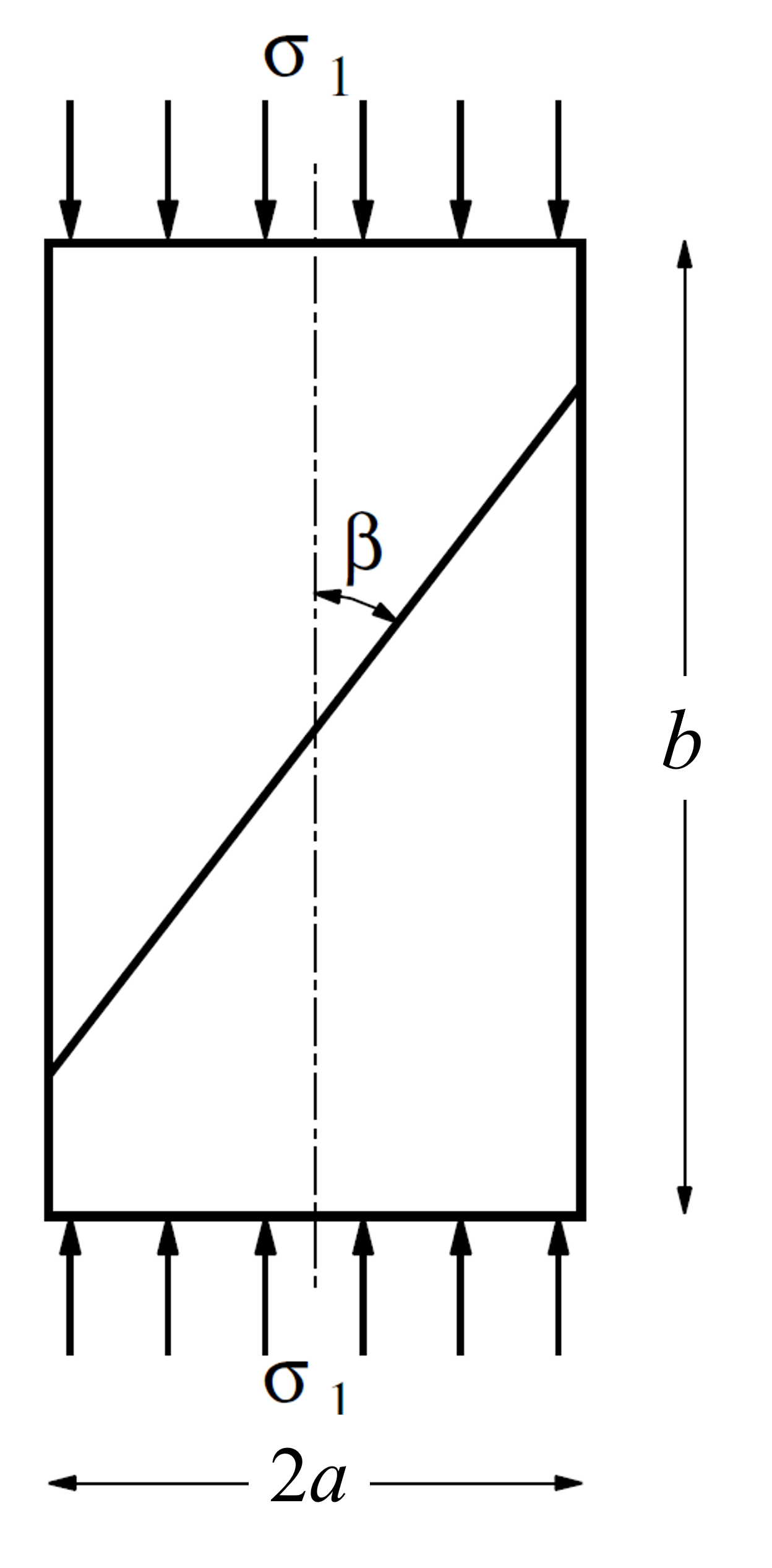
Figure 1: Problem geometry.

Analytical Prediction

As a definition, let

\[\kappa = 1 - \tan(\phi_j) \tan(\beta)\]

in which \(\beta\) is the weak-plane angle, as indicated in Figure 1. Before failure occurs, the state of stress is homogeneous in the sample. Failure will be initiated on the weak plane when, for \(\kappa >\) 0,

\[-\sigma_1 = {{2 c_j}\over{\kappa \sin 2\beta}}\]

provided the value \(-\sigma_1\) of the compressive strength (tension positive) does not violate the Mohr-Coulomb failure criterion,

\[-\sigma_1 = 2 c \sqrt N_{\phi}\]

in which

\[N_{\phi} = {{1 + \sin\phi}\over{1 - \sin\phi}}\]

If this criterion is violated, or if \(\kappa \leq\) 0, failure will occur in the matrix instead, on planes inclined at an angle of \((\pi/4 - \phi/2)\) with respect to the axis of symmetry of the sample. See Jaeger and Cook (1979) for details.

3DEC Model

For the numerical simulation, a cylinder with a radius of 1 m and height of 4 m is selected. A system of reference axes with the \(x\)- and \(y\)-axes located in the base of the cylinder and the \(z\)-axis pointing along the cylinder axis is selected. This domain is discretized into tetrahedral zones (see Figure 2). Nodel mixed discretization is used to get more accurate plasticity for the tets (block zone nodal-mixed-discretization). A uniform velocity is applied in the \(z\)-direction at both ends of the cylinder to induce compression of the sample.

The effect of the variation of \(\beta\) has been studied every five degrees from 0° to 90°. The input file uses a FISH function (solveAll) to calculate the compressive strength at each \(\beta\) value. These are stored in a table that is not cleared with the model new command since the skip table keywords are added. The final vertical stress calculated with FISH function sigmav is added to a table at the end of each run. This approach allows us to save the whole parametric analysis in one file. For each value of \(\beta\), cycling continues until an accumulated displacement of 4.5e-4 is reached (using the FISH function halt), indicating enough total strain to cause failure at all angles.

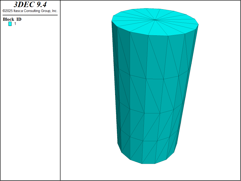
Figure 2: 3DEC grid — uniaxial compressive strength test.

Results and Discussion

Figure 3 compares results of the 3DEC runs with the analytical compressive strength predictions. The match is satisfactory, with a relative error smaller than 3% for all values of \(\beta\).

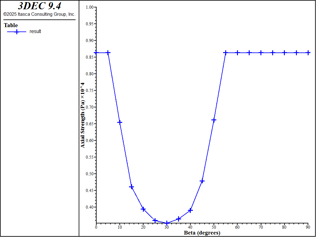
Figure 3: Compressive strength comparison.

Reference

Jaeger, J. C., and N. G. W. Cook. Fundamentals of Rock Mechanics, 3rd Ed. New York: Chapman and Hall (1979).

Data Files

UniaxialStrengthJointed.dat

;---------------------------------------------------------------------
; compression test of cylindrical sample using
;   ubiquitous joint model
;---------------------------------------------------------------------
model new

; FISH functions used to support  - 
; the strength calculation and the halt function
fish define sigmav
    local gps = block.gp.list( block.gp.isgroup(::block.gp.list,'bottom') )
    return list.sum(block.gp.force.reaction(::gps)->z)/3.06147
end
; Function that determines if solving should stop
fish define halt
    global gpHalt
    halt = block.gp.disp(gpHalt)->z > 4.5e-4
end

; The main function 
fish define solveAll
    global result = list
    ; Check angles from 0-90 in 5 degree increments
    loop local beta (0,90,5) 
        command
            model new skip table ; Reset model state, FISH preserved by default
            model random 10000
            model large-strain off
            fish automatic-create off
            
            ; Create the geometry
            block create drum center-1 0,0,0 center-2 0,0,4 radius-1 1 radius-2 1 edges 16
            block zone generate-new minimum-edge 1 maximum-edge 1
            block gridpoint group 'top' range position-z 4
            block gridpoint group 'bottom' range position-z 0
            
             ; Assign model and properties
            block zone cmodel assign ubiquitous-joint
            block zone property density 2500 bulk 1e8 shear 7e7 cohesion 2e3
            block zone property friction 40 dilation 0 tension 2400
            ; dip is 90 degrees off of beta
            block zone property dip [90 - beta] dip-direction 0 joint-cohesion 1e3 
            block zone property joint-friction 30 joint-dilation 0 ...
                          joint-tension 2000
                          
            ; Assign boundary conditions
            block gridpoint apply velocity-z -0.001 range group 'top'
            block gridpoint apply velocity-z 0.001 range group 'bottom'
            
            ; turn on NMD for accuracy
            block zone nodal-mixed-discretization on
                       
            ; Cycle till the target strain is reached
            [global gpHalt = block.gp.near(0,0,0)]
            model solve fish-halt [halt]
            
            ; Add results to table
            table 'result' add ([beta],[sigmav])
        end_command
    end_loop
end
; Run all 18 cases
[solveAll]

; Save the last state, and the accumulated table
model save 'final'

Endnote

[1]

This example is listed under the present document title in the i Examples dialog (use the menu command Help -> Examples… to access).