Bonded-Particle Modeling

The PFC model provides a synthetic material consisting of an assembly of rigid particles that interact at contacts and includes both granular and bonded materials. This synthetic material encompasses a vast microstructural space, and only a small portion of this space has been explored. The bonded-particle modeling methodology provides a rich variety of microstructural models in the form of bonded materials (Potyondy et al. [2025)]; Potyondy [2015]; Potyondy and Cundall [2004]). In a bonded-particle model (BPM), the microproperties include stiffness and strength parameters for the particles and bonds. Damage is represented explicitly as broken bonds, which form and coalesce into macroscopic fractures when loaded (see Figures 1 and 2). The modeling methodology has been applied extensively to model a variety of rock mechanics problems.[1]

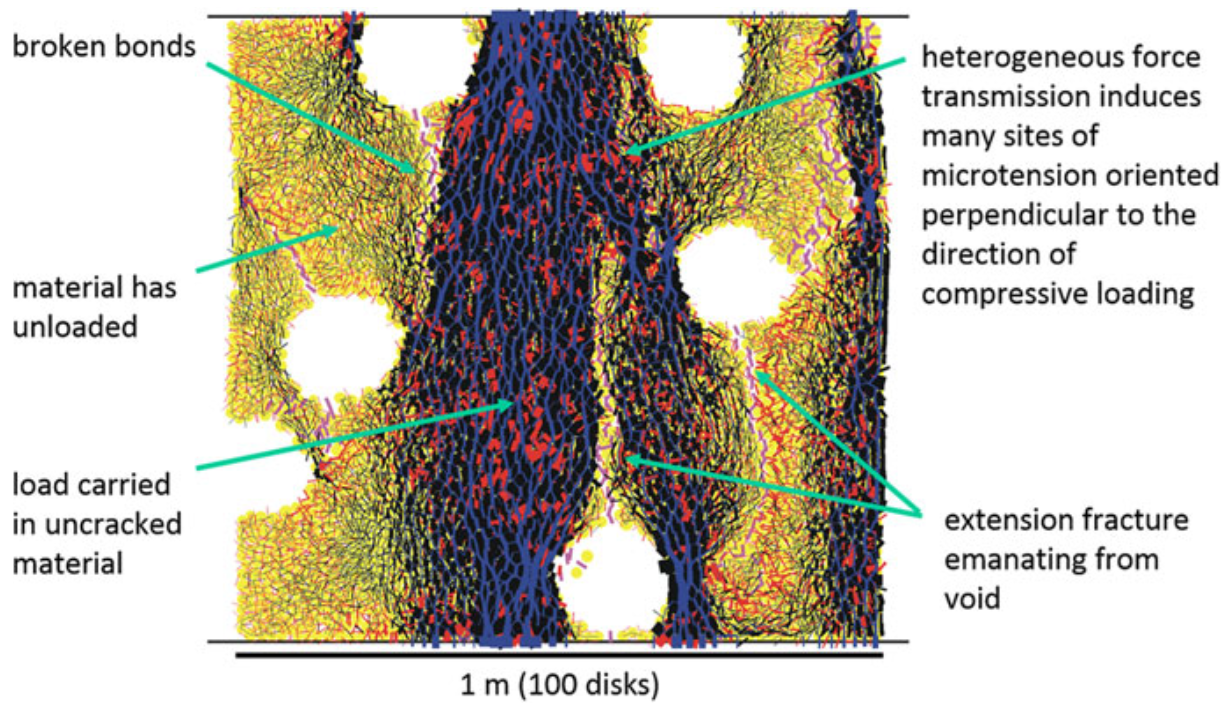
Figure 1: A two-dimensional bonded-particle model consisting of a packed assembly of rigid disks joined by deformable and breakable cement at particle-particle contacts in the post-peak region of a UCS test. Blue and black denote compression and red denotes tension. (From Fig. 3 of Potyondy [2015])

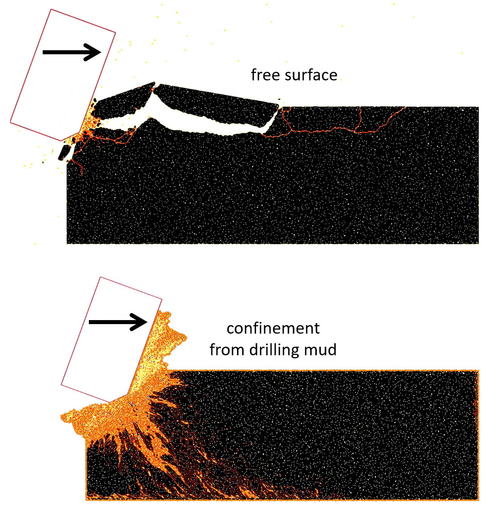
Figure 2: PFC2D model of a rock-cutting test for both dry and wet cutting, during which two cutters are moved across the surface of the synthetic rock, while monitoring forces on the cutters, damage in the rock, and all energy quantities of the cutter-rock system. Wet cutting is modeled by applying a confining pressure to the evolving rock surface via the chaining algorithm. The chaining algorithm repeatedly identifies a connected chain of particles on the rock surface and applies an external force to each of these particles based on the local chain geometry and specified pressure.

BPMs are a subset of the space of models encompassed by the PFC model; thus, the essential features of the PFC model are summarized in the first subsection. Potyondy (2015) provides a comprehensive definition of the BPM as of 2015.[2] The definition is expanded in the second subsection wherein the BPM is situated within the broader context of microstructural rock models, of which it is one example. The third subsection describes the sorts of bonded-particle materials that can be constructed with the PFC model. The materials are described in terms of the microstructures that they mimic. The fourth subsection describes the modeling philosophy that underlies both the development and application of BPMs. The fifth subsection lists tutorials and examples that demonstrate modeling operations required to build BPMs. The final subsection presents the material-modeling support package that supports creation of bonded materials.

PFC Model Essentials

The essential features of the PFC model are summarized here. The features include the model components, timestep scaling, local damping, how static equilibrium is determined, how force chains are visualized, and how a particle size distribution is measured. All of these items should be understood by a user of PFC.

Model Components

Components of the PFC model are described here.

Timestep Scaling

The PFC model can be run in either dynamic or timestep-scaling mode. The model runs in dynamic mode unless timestep scaling is activated. When run in dynamic mode, the true dynamic response of the system is obtained.

Timestep scaling may be used to reach the steady-state condition (for which all particle accelerations are zero, corresponding to either static equilibrium or steady flow) with as few computational cycles as possible. When timestep scaling is active, a fictitious inertial mass is calculated for each particle such that its stable timestep is one, thereby giving all degrees of freedom in the system an equal time response. Time can be thought of as a relaxation time required to reach the steady-state condition so that the timestep has units of length per step. The path to the steady-state condition is unphysical in the sense that the inertial masses [3] and velocities have been scaled to achieve rapid convergence.[4] Only the final steady-state condition is valid, and transitory states do not represent the true dynamic behavior of the system. For path-dependent phenomena that involve formation of mechanisms, this may result in an incorrect steady-state condition. A thorough discussion of timestep scaling is provided in Timestep Scaling.

Local Damping

Kinetic energy can be dissipated by frictional sliding and viscous damping (dashpots at contacts); however, these dissipation mechanisms may not be sufficient to arrive at a steady-state condition in a reasonable number of cycles. Local damping is a particle-based damping scheme to remove additional kinetic energy. Local damping acts on each particle, applying a damping force with magnitude proportional to the unbalanced force. The proportionality coefficient is called the local-damping coefficient that is set by the ball attribute damp (or clump/rblock) commands. Local damping is deactivated by setting the local-damping coefficients of all particles to zero, which is the default state.

For compact particle assemblies, local damping may be used to establish static equilibrium and to conduct quasi-static deformation simulations (and for most models, quasi-static conditions are maintained by setting the local damping coefficient to 0.7). When a dynamic simulation of a compact particle assembly is required, contact-model based damping strategies are preferred and the local-damping coefficient should be set to zero or a small value. Local damping is not appropriate for particles in free fall because it applies a damping force that acts opposite to the unbalanced force \((mg)\) where \(m\) is particle mass, thereby making the particle acceleration less than the gravitational acceleration \((g)\). If the simulation is dominated by rapid impacts, one should consider the use of a hysteretic contact model for realistic dissipation of energy. A thorough discussion of damping is provided in Mechanical Damping.

Static Equilibrium

If one were to continue cycling after static equilibrium is obtained, then there would be no further change in the model configuration. The proximity to static equilibrium is estimated by the mechanical ratio average

(1)\[\epsilon_{\rm arat} = { {\rm avg}( || \mathbf{F_{ub}} || ) \over {\rm avg}( F_{\rm int} ) } = { \sum_n \bigl( ||\mathbf{F_c} + \mathbf{F_a} + \mathbf{F_b}|| \bigr) / n \over \sum_n \bigl( ||\mathbf{F_c}|| + ||\mathbf{F_a}|| + ||\mathbf{F_b}|| \bigr) / n }\]

The ratio-average is the average (over all \(n\) particles) unbalanced force magnitude divided by the average (over all \(n\) particles) force intensity. The unbalanced force is the vector sum of all forces acting on the particle (contact, applied and body), and the force intensity is the sum of the force magnitudes. In the above expression, vector magnitude is defined by

(2)\[|| \mathbf v || = \sqrt{v_x^2 + v_y^2 + v_z^2}\]

and only free translational degrees-of-freedom are used in the computations.

A model is run to a state of static equilibrium with the model solve mechanical ratio-average command such that the model will continue to cycle until

(3)\[\varepsilon_{\rm arat} \leq \varepsilon_{\rm lim}\]

For most models, static equilibrium corresponds with

(4)\[\epsilon_{\rm lim} \in [10^{-5},10^{-4}]\]

Force-Chain Fabric

The PFC model carries load via force chains that propagate from one particle to the next across particle-particle contacts. The PFC3D force-chain fabric is depicted as a network of cylinders, with a cylinder at each contact. Force magnitude corresponds with cylinder thickness, and force direction corresponds with cylinder orientation. The force-chain fabric can be displayed as either bicolored to denote compression and tension or scale-colored to denote magnitude (see Figure 3). Both displays are provided by the contact plot item. The bicolored display is obtained by specifying: {Shape: Cylinder}, {Color By: Text Val: force chain}, {Color Opt: Named}, {Scale by Force: checked}, and {Directed: checked}. The scale-colored display is provided by specifying: {Shape: Cylinder}, {Color By: Vector Qty: force, Qty: Mag}, {Color Opt: Scaled}, {Scale by Force: checked}, and {Directed: checked}.

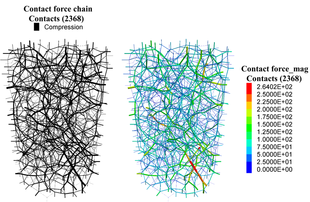
Figure 3: Force-chain fabric in the PFC3D linear material packed in a cylindrical vessel at 150 kPa pressure showing: bicolored (left) and scale-colored (right) displays. The linear material cannot sustain tension; therefore, the bi-colored display shows only compression.

Particle Size Distribution

The cumulative distribution of particle size is most often used to characterize particulate media (Santamarina et al., 2001). The typical particle size distribution curve is a cumulative distribution of mass according to particle size — it is NOT a cumulative distribution of particle counts. The curve expresses the mass percentage of particles that can pass through a given sieve size. The horizontal axis is particle size, and the vertical axis is “mass percent passing.” A typical particle size distribution curve is shown in Figure 4. If the vertical axis is labelled “percent finer than,” then it is understood that this denotes the percentage by mass, not the percentage by number. The equivalent particle sizes corresponding to selected percentiles are frequently quoted. For example, \(d_{50}\) corresponds to the particle size that 50 percent of the particles are finer than (and these particles comprise 50 percent of the total mass), and \(d_{10}\) corresponds to the particle size that 10 percent of the particles are finer than (and these particles comprise 10 percent of the total mass). The quantity \(d_{50}\) is called the median particle size. The extent/slope and convexity or concavity of the particle size distribution curve are characterized by the coefficients of uniformity \((C_u)\) and curvature \((C_c)\) where

(5)\[C_u = {d_{60} \over d_{10}} \quad {\rm and} \quad C_c = {d_{30}^2 \over d_{10}d_{60}}\]

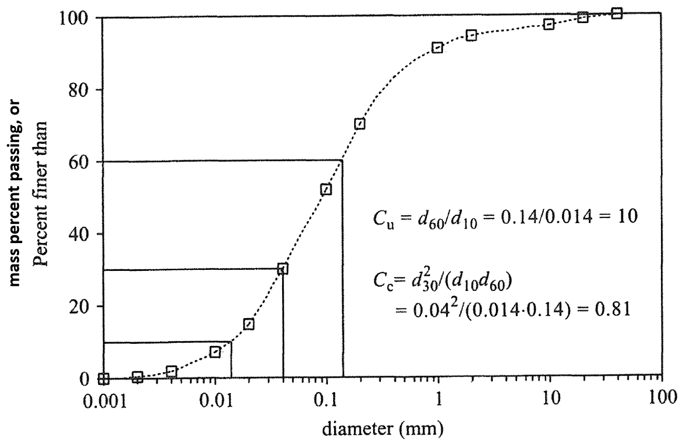
Figure 4: Typical particle size distribution curve showing the cumulative distribution of mass according to particle size. (From Fig. 2.10 of Santamarina et al. [2001])

A well-graded particulate mass consists of a broad range of particle sizes, where larger particles form the structural skeleton — supporting the primary force chains typically aligned with the direction of maximum principal stress — and smaller particles occupy the voids between them. These smaller particles enhance lateral confinement and help prevent buckling of the force chains under load. This arrangement allows well-graded materials to achieve higher packing density and improved mechanical stability compared to poorly graded ones.

According to the Unified Soil Classification System (USCS), as defined in ASTM D2487 (ASTM [2020]), a coarse-grained soil is considered well-graded if its particle size distribution meets the following criteria:

• For gravel-dominated soils: \(Cu > 4\) and \(1 < C_c < 3\). Gravel has particle sizes that range from 4.75 mm to 76.2 mm.

• For sand-dominated soils: \(Cu > 6\) and \(1 < C_c < 3\). Sand has particle sizes that range from 0.075 mm to 4.75 mm.

The particle size distribution of the PFC model can be computed by the FISH functions in Potyondy (2025a). The volume percent passing curve can also be obtained with the measurement logic (by specifying the number of bins and the particle-diameter range for the size-distribution computation when creating a measurement circle/sphere with the measure create bins command and extracting the information into a table with the measure dump command). If all sampled particles have the same density, then the volume percent passing curve is equal to the mass percent passing curve.

Microstructural Rock Models (BBM, FDEM, and BPM)

Rock can be modeled as a continuum or bonded assembly of discrete particles (see Figure 5). We use the term microstructural rock model to refer to any discrete model that can mimic rock microstructure at the grain scale. Continuum models enforce continuous behavior via constitutive relations that describe the stress-strain response occurring within finite-sized material regions (elements or zones). Discrete models enforce particulate behavior via contact (or interface) models that describe the force-displacement and moment-rotation relations at the particle-particle contacts. Discrete models provide an explicit microstructure of cemented particles for which the particle size, shape and packing as well as the particle and cement properties (e.g., stiffness, strength, degree of cementation) can be varied. The constitutive response of a discrete model is an emergent property arising when the contact forces and particle displacements are averaged over a representative volume of particles to obtain stress and strain, respectively. The finite-discrete element method (Munjiza, 2004) combines both continuum and discrete formulations to provide a rock model that starts out as an elastic continuum and then transforms into a discrete model as cohesive elements break.

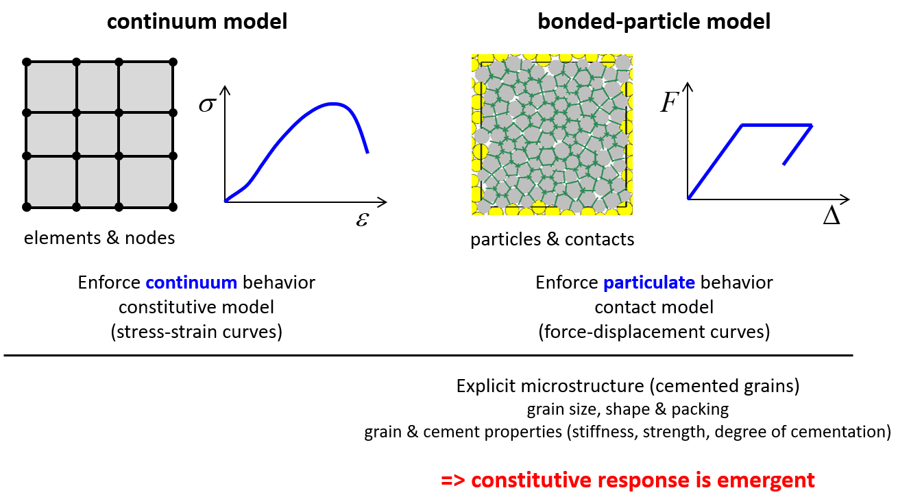
Figure 5: Comparison of continuum and discrete (bonded-particle) models.

Microstructural rock models can be thought of in the following ways: (1) the individual elements are not rock grains, in which case the model captures the behavior (that includes damage formation) within a macroscopic region — such models have element sizes much, much larger than rock grains; (2) the individual elements are rock grains, in which case the model captures the behavior as above, but also captures the grain-scale micromechanisms at the true grain scale — such models have element sizes equal to those of the rock grains; and (3) agglomerates of individual elements represent grains, in which case the model captures grain crushing and material heterogeneity at a larger scale than the individual elements.

Three common microstructural rock models are described and compared with one another as follows.

• Bonded-block models (BBMs) consist of a perfectly interlocked mesh of elastoplastic, unbreakable, polyhedral blocks (typically tetrahedrons or Voronoi cells) joined by bonds at block-block interfaces and modeled with the UDEC and 3DEC codes. A bond breaks when the stress it is carrying exceeds the material strength, and then a Coulomb-type friction is applied to the broken interface (Garza-Cruz and Pierce, 2014; Sinha and Walton, 2020). Mechanical behavior is simulated by the distinct-element method. BBM material mimics the microstructure of angular, interlocked, elastoplastic blocks with interfaces that can sustain partial damage (because an interface consists of bonded subcontacts that can break independently of one another). Blocks remain interlocked even after the bonds at all interfaces along the block boundary have broken. The synthetic material is initially an elastoplastic continuum with a network of potential failure planes at the bonded interfaces, and as the bonded subcontacts at the interfaces break, the continuum transforms into a collection of discrete polyhedral bodies. A typical bonded-block model is shown in Figure 6.

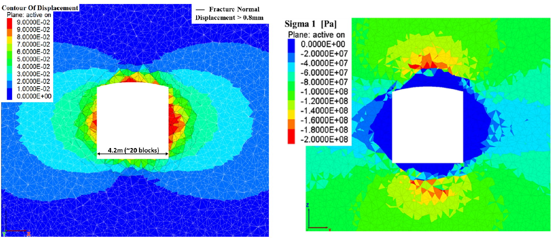
Figure 6: Tunnel response at depth of a 3DEC bonded block model after being subjected to a caving-induced loading and unloading cycle. Displacement contour (left image) shows high bulking near the excavation surface. As stresses redistribute, surface-parallel fractures form and coalesce to create debonded fragments, resulting in an inner shell of highly damaged ground with a 2-m thickness. Fractures with normal displacement greater than 0.8 mm are shown as black lines. Rapid confinement build-up outside the inner shell allows the rock mass to sustain high induced stress concentrations (right image). (From Figs. 11 and 13 of Garza-Cruz et al. [2014])

• Hybrid finite-discrete element models (FDEMs) consist of a perfectly interlocked mesh of elastic, unbreakable, tetrahedral finite elements joined by cohesive elements at element-element interfaces. A cohesive element breaks after having dissipated the material fracture energy, and then a Coulomb-type friction is applied to the broken interface (Mahabadi et al., 2012; Lisjak and Grasselli, 2014). Mechanical behavior is simulated by the finite-discrete element method that blends finite-element techniques with discrete-element concepts and with impenetrability between elements enforced by a penalty function method (Barla and Beer, 2012). FDEM material mimics the microstructure of angular, interlocked, elastic tetrahedrons with interfaces that may sustain partial damage (as the interface yields after having reached its peak strength). Tetrahedrons remain interlocked even after the material fracture energy at all interfaces along the tetrahedron boundary has been dissipated. The synthetic material is initially an elastic continuum with a network of potential failure planes at the element interfaces, and as the cohesive elements at the interfaces soften and break, the continuum transforms into a collection of discrete tetrahedral bodies. A typical hybrid finite-discrete element model is shown in Figure 7.

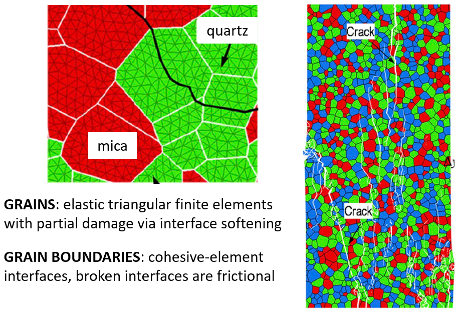
Figure 7: FDEM grain-based model (2D), showing mineral grains (left), and damage (broken cohesive-element interfaces) at end of UCS test (right). (From Figs. 7 and 11 of Li et al. [2020])

• Bonded-particle models (BPMs) consist of a packed — but not necessarily perfectly interlocked — assembly of rigid, unbreakable particles (spheres, clumps [overlapping spheres that behaves as a rigid body] or polyhedra) joined by bonds at particle-particle interfaces and modeled with the PFC codes. A bond breaks when the stress it is carrying exceeds the material strength, and then a Coulomb-type friction is applied to the broken interface (Potyondy [2015]; Potyondy and Cundall [2004]). Mechanical behavior is simulated by the distinct-element method. BPM material can mimic a variety of microstructures by using different contact models to provide different interface geometry, force-displacement/moment-rotation response, and post-breakage behavior (see Bonded-Particle Materials). The synthetic material is initially a bonded-particle assembly with a network of potential failure planes at the particle-particle interfaces, and as these interfaces break, the bonded-particle assembly transforms into a collection of discrete particles. A typical bonded-particle model is shown in Figure 1.

The mechanical behavior of these microstructural models ranges from that of a solid material when bonds or cohesive elements are intact to that of a granular material when bonds or cohesive elements have all broken. If individual grains or other microstructural features are modeled as agglomerates of either bonded blocks, FDEM elements, or bonded particles, then grain crushing and material heterogeneity at a larger scale than the blocks, elements, or particles can also be accommodated by these models, which are called grain-based models (GBMs, Potyondy [2010]). Because the blocks and elements of the BBM and FDEM materials are not grains, then only when this grouping process is done, do these models become true microstructural models that can mimic rock microstructure at the grain scale. Example of grain-based models are shown in Figures 7, 8, and 9.

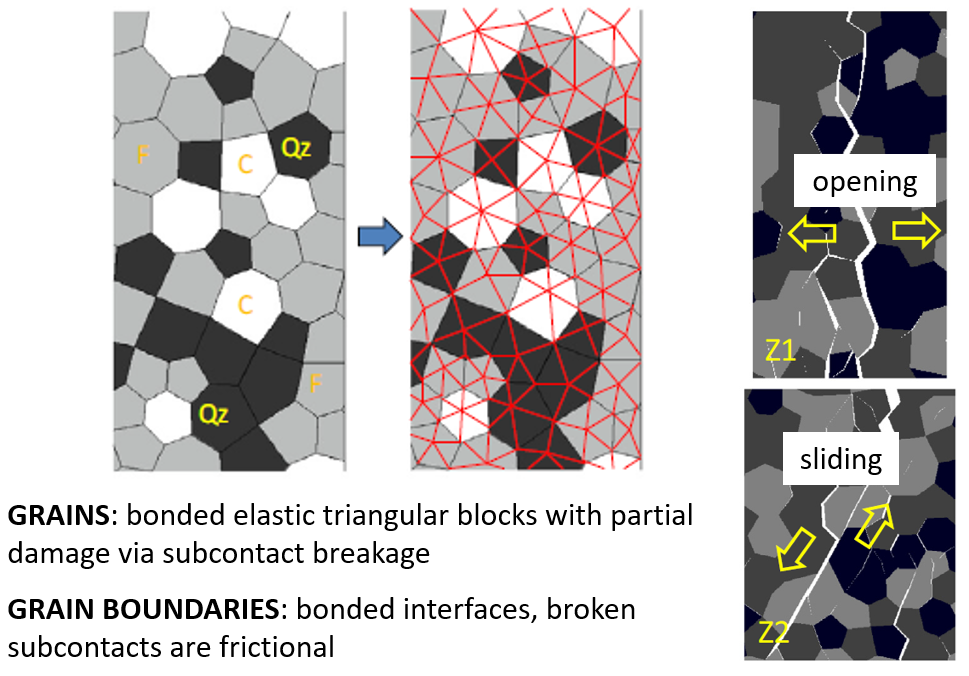
Figure 8: BBM grain-based model (2D, UDEC), showing mineral grains (left), and damage (broken interfaces) at end of UCS test (right). (From Figs. 2 and 7 of Gao et al. [2016])

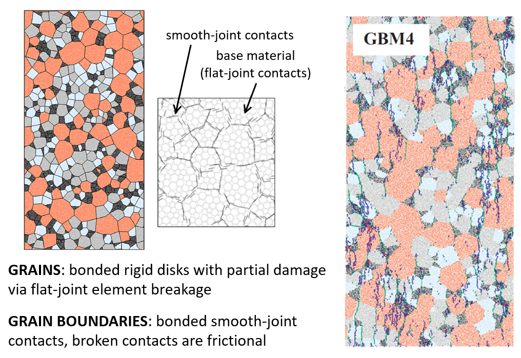
Figure 9: BPM grain-based model (2D, PFC2D), showing mineral grains (left), and damage (broken bonds) at end of UCS test (right). (From Figs. 11 and 19 of Zhou et al. [2019])

Bonded-Particle Materials

Bonded-particle materials are analogous to rock, which can be viewed as an aggregate of crystals and amorphous particles joined by varying amounts of cementing materials (see Figure 10). BPM material can mimic a variety of microstructures by using different contact models to provide different interface geometry, force-displacement/moment-rotation response, and post-breakage behavior.[5]

• The contact bond contact model provides the behavior of an infinitesimal (zero area), linear elastic, and either bonded or frictional interface that carries a force (see this figure). The contact-bonded material (defined in Section 2.5 of Potyondy [2025a]) mimics the microstructure of spot-welded (without moment resistance), unbreakable, rigid particles (see Figure 11).

• The parallel bond contact model provides the behavior of two interfaces: an infinitesimal (zero area), linear elastic with no tension, and frictional interface that carries a force; and a finite-size (nonzero area), linear elastic, and bonded interface that carries a force and moment — after bond breakage, the second interface is removed along with the force and moment that it carries such that the interface no longer resists moment (see this figure). The parallel-bonded material (defined in Section 2.6 of Potyondy [2025a]) mimics the microstructure of cemented (with moment resistance) unbreakable, rigid particles (see Figure 11).

• The soft bond contact model is like the parallel bond contact model, but instead of failing in a brittle fashion, the bond softens after reaching its peak strength (see Figures 12 and 13). The soft-bonded material is defined in Section 2.7 of Potyondy (2025a).

• The flat joint contact model provides the behavior of a finite-size (nonzero area), linear elastic, and either bonded or frictional interface that may sustain partial damage — even after all bonded elements at the interface have broken, the interface continues to resist moment (see this figure). The flat-jointed material (defined in Section 2.8 of Potyondy [2025a]) mimics the microstructure of angular, interlocked, rigid particles with interfaces that may sustain partial damage, and with particles that remain interlocked even after the bonded elements at all interfaces along the particle boundary have broken (see Figure 14 as well as figures A and B).

• The subspring network contact model provides the behavior of a finite-size (nonzero area), linear elastic, and either bonded or frictional interface that may sustain partial damage. The subspring network contact model is combined with a grain-breakage scheme to provide the Subspring Network contact model with rigid, Breakable, Voronoi-shaped grains (SNBV model, Potyondy et al. [2025]). The SNBV material (defined in Section 1.3 of Potyondy [2025c]) mimics the microstructure of angular, interlocked, breakable grains with interfaces that may have an initial gap and can sustain partial damage (see Figure 15).

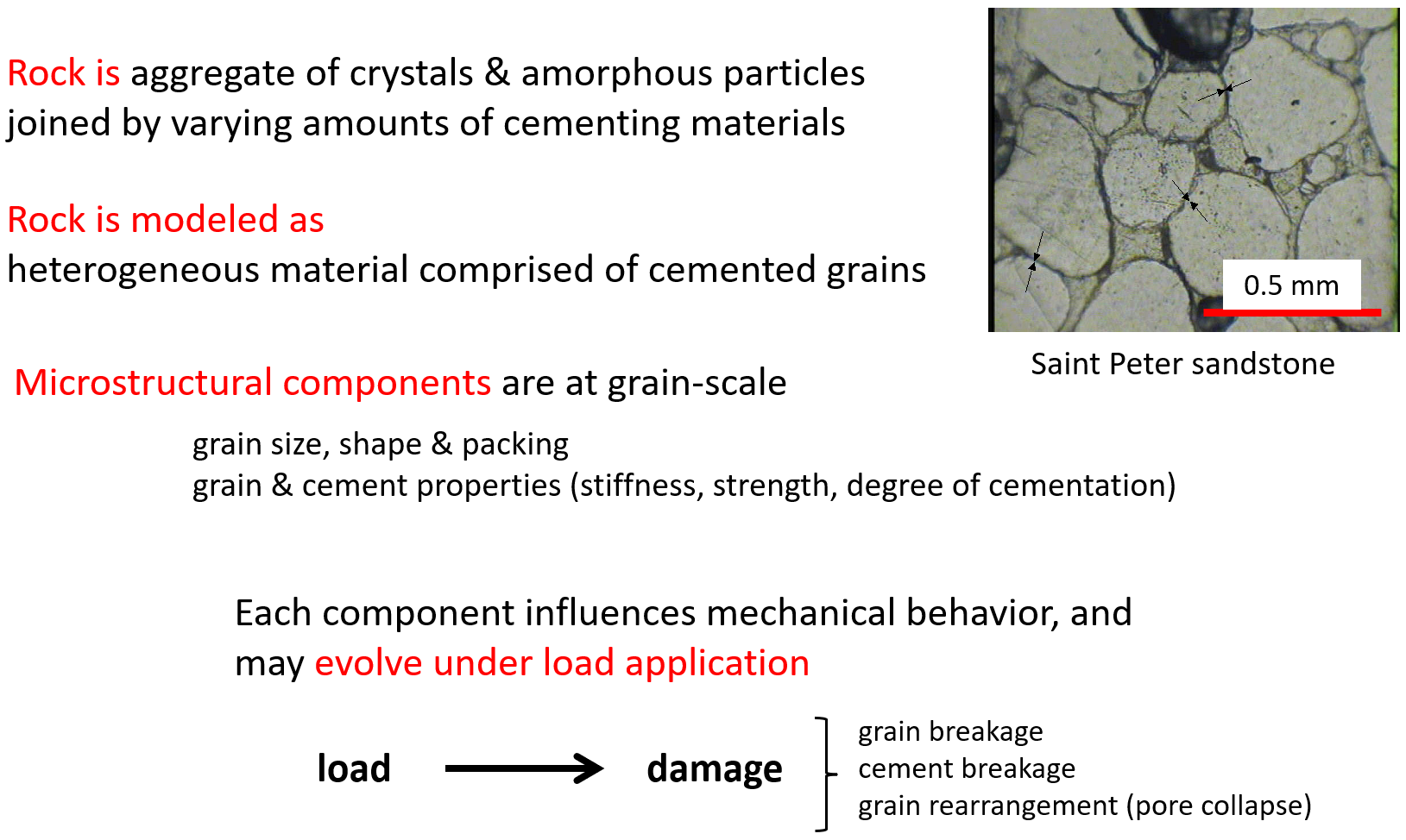
Figure 10: Microstructural physics of rock and how it can be modeled as a bonded-particle material.

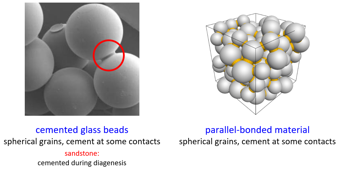
Figure 11: Parallel-bonded material. The contact-bonded material behaves like a parallel-bonded material in which the parallel-bond radii are near zero.

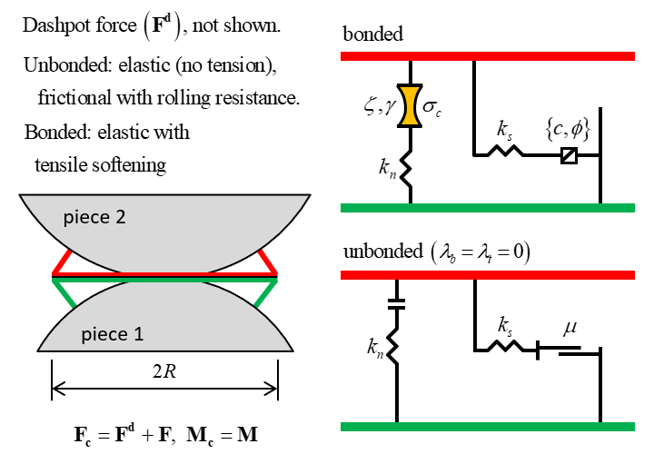
Figure 12: Behavior and rheological components of the soft bond model with friction multipliers of zero and inactive dashpots.

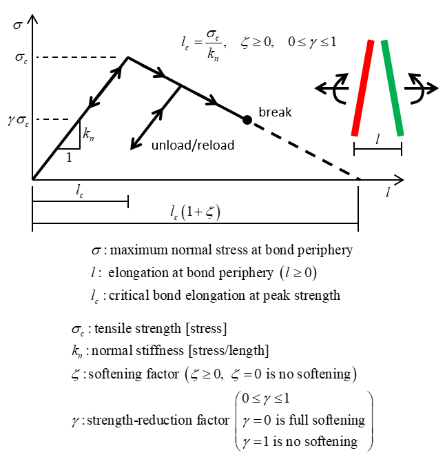
Figure 13: Softening behavior of the soft bond model.

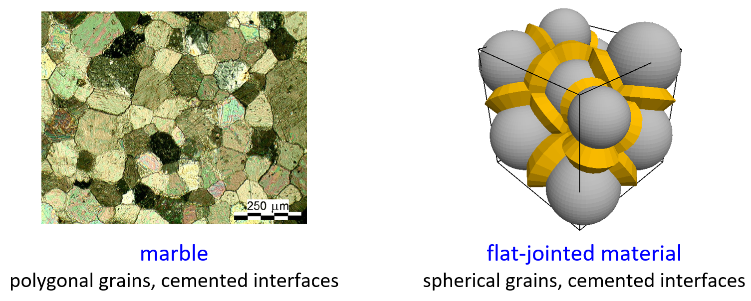
Figure 14: Flat-jointed material.

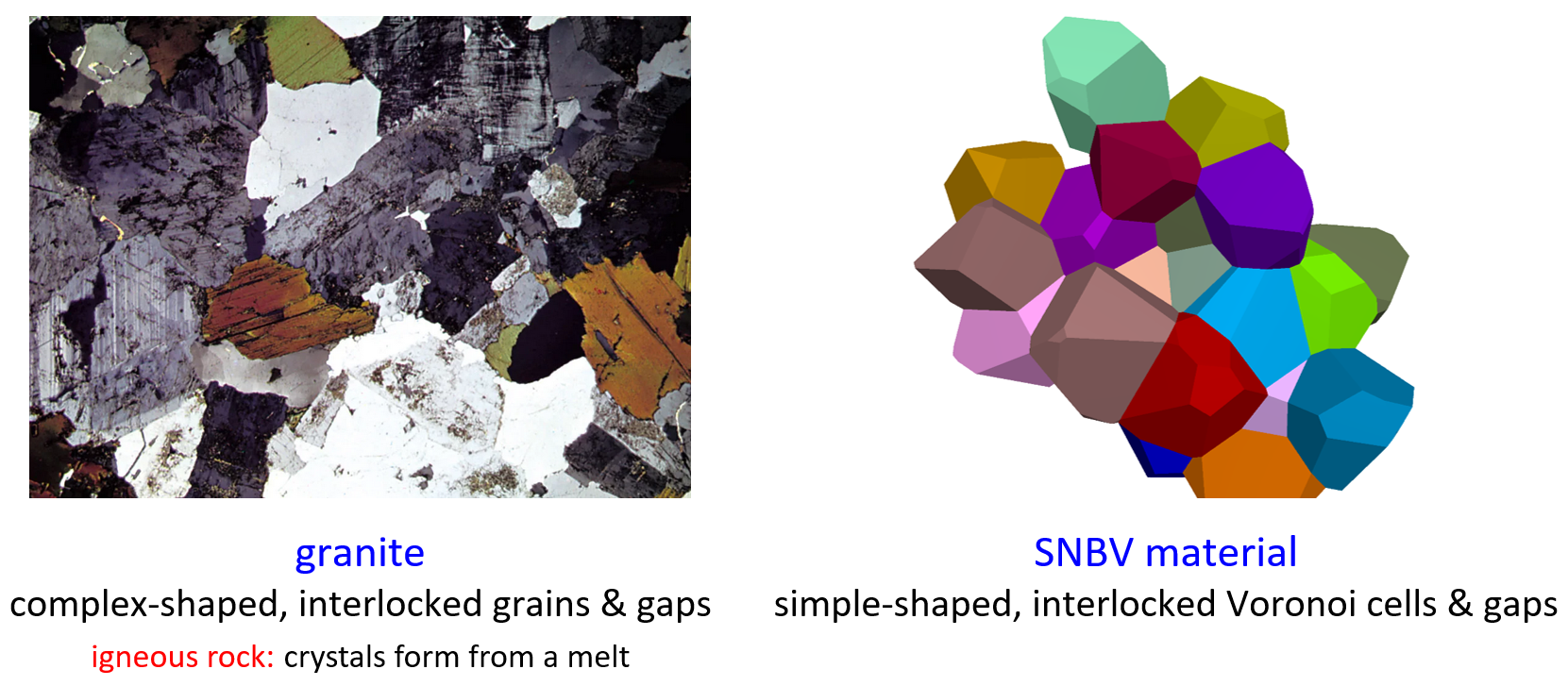
Figure 15: Subspring Network Breakable Voronoi (SNBV) material.

Modeling Philosophy

The modeling philosophy that underlies both the development and application of the PFC model (and which includes the importance of having a well-defined model of a system, and the limitations of any such model) is well stated in the following excerpt from the chapter “Models and Their Limitations” in a book about the physics of baseball.

In his analysis of a real system, a physicist constructs a well-defined model of the system and addresses the model. The system we address here is baseball… We cannot calculate from first principles the character of the collision of an ash bat with a sphere made up of layers of different tightly wound yarns, nor do we have any precise understanding of the effect of the airstream on the flight of that sphere, with its curious yin-yang pattern of stitches. What we can do is construct plausible models of those interactions that play a part in baseball that do not violate basic principles of mechanics. Though these basic principles … severely constrain such models, they do not completely define them. It is necessary that the models touch the results of observations — or the results of the controlled observations called experiments — at some points so that the model can be more precisely defined and used to interpolate between known results, or to extrapolate from them… If the model is well chosen, so as to represent the salient points of the real system adequately, conclusions derived from an analysis of the model can apply to the system to a useful degree. (Adair, 2002, pp. 1–2)

A modeling philosophy addresses the essential question: Why are we modeling this problem, and what can we expect to learn from the model? This question must be answered by each modeler, because no model is complete or fully verifiable (Oreskes et al., 1994); instead, the best that can be done is to sanction the model. According to Winsberg (2010, p. 23):

The sanctioning of simulations does not cleanly divide into verification and validation. In fact, simulation results are sanctioned all at once: simulationists try to maximize fidelity to theory, to mathematical rigor, to physical intuition, and to known empirical results. But it is the simultaneous confluence of these efforts, rather than the establishment of each one separately, that ultimately gives us confidence in the results.

PFC models for rock have been sanctioned by demonstrating that they match the response obtained during tension and compression tests of typical rocks. The response consists of the properties measured during such tests as well as the microstructural behavior that occurs during such tests. In some cases, the BPM microproperties are chosen to approximate the true microstructural properties (in which case, the model is called a bonded-grain model[6]), and then the macroscopic behavior is studied. But in most cases, either the true microstructural properties are not known, or the BPM is a simplification of the true microstructural features. In such cases, the BPM microproperties must be chosen by performing a calibration process in which a particular instance of a BPM is used to simulate a set of material tests, and the BPM microproperties are chosen to reproduce the relevant response occurring in such tests. In addition to the laboratory-scale tests noted above, field-scale tests that may include excavation-induced damage have also been used in the sanctioning process (Potyondy et al., 2024).

Further discussion of the sanctioning of PFC models is provided in Potyondy et al. (2025) and Potyondy (2015), and further discussion of modeling philosophy is given in Starfield and Cundall (1988), Starfield (1997), and Nicolson et al. (2002).

Bonded-Particle Modeling Examples

The following tutorials and examples are related to bonded-particle modeling. They illustrate modeling operations required to build, test, and monitor damage in BPMs. Most of these capabilities are provided by the Material Modeling Support Package. The creation of a parallel-bonded material is illustrated in the Generating a Bonded Assembly tutorial. The Using the CMAT tutorial discusses the issue of specifying the cmat.proximity and the bonding gap appropriately to bond contacts with a desired contact gap. The Inclusions in a Matrix tutorial creates a bonded material with spatial heterogeneity of contact properties. The Creation of a Synthetic Rock Mass (SRM) Specimen tutorial describes the insertion of smooth-jointed interfaces into a parallel-bonded material. The Fragmentation example creates a parallel-bonded material and performs an unconfined compression test on the specimen until complete failure; this example also illustrates how bond breakage and fragments can be monitored during the simulation. The Rock Testing example compares the mechanical response of parallel-bonded and flat-jointed materials under unconfined compression and direct-tension tests.

Material Modeling Support Package

The Material Modeling support package (mmPkg, Potyondy [2025a]) provides a consistent set of FISH functions to support creation of PFC2D and PFC3D materials (granular and bonded) in various material vessels followed by laboratory testing to measure mechanical properties and observe microstructural behavior while tracking and visualizing material damage. The models support practical applications via boundary-value models made from these materials and scientific inquiry via further exploration of the microstructural space provided by the PFC model.

Bonded materials are analogous to rock, which can be viewed as an aggregate of crystals and amorphous particles joined by varying amounts of cementing materials (see Figure 10). A rich variety of microstructures can be produced by modifying the bonded material itself. Such microstructures are obtained either by modifying the properties of the particles and cement or by modifying the packing fabric. The particle properties are size and shape. The cement properties are deformability and strength as well as evolving damage. The cement properties are embodied in the contact model, but the macroscopic material behavior is also sensitive to the ways in which new contacts form and contacts deemed to be broken behave. The packing fabric at the time of bond installation affects the macroscopic properties of the synthetic material because bonds can be installed only at existing contacts — more bonds give increased stiffness and strength. The mmPkg provides a well-defined and controlled procedure (pack the particles to a specified pressure and then install bonds between all particles that are within a specified distance of one another) to create BPMs.

The mmPkg provides: a material-genesis procedure to create six types of materials; well-defined sets of microproperties to define each material; testing procedures to perform standard rock-mechanics laboratory tests upon the materials; microstructural monitoring to measure microstructural properties, visualize the microstructure, and measure and visualize material damage in the form of bond breakages; and examples of the creation and testing of each material. A concise summary of the package capabilities follows.

Material genesis of granular materials (linear and Hill[7]) and bonded materials (contact-bonded, parallel-bonded, soft-bonded, and flat-jointed) in polyaxial, cylindrical, and spherical physical vessels or polyaxial periodic vessel. Material particles can be balls or clumps, and 3D flat-jointed materials of spherical, Voronoi or tetrahedral particles. Stress can be installed into the finalized periodic ensemble (after bonding), and then this ensemble can be converted into a periodic brick which is assembled into a larger geometric shape. Material tests are compression (confined, unconfined, and uniaxial strain), diametral compression, and direct tension. Microstructural monitoring includes properties (such as particle size distribution) with microstructural plots and crack monitoring for bonded materials.

Please visit our website at http://www.itascacg.com/material-modeling-support to download the material-modeling support package.

The Subspring Network contact model with rigid, Breakable, Voronoi-shaped grains (SNBV model) is a type of bonded-particle model that mimics the microstructure of angular, interlocked, breakable grains with interfaces that may have an initial gap and can sustain partial damage (Potyondy et al. [2025]; Potyondy and Fu [2024]). Support for creation and laboratory testing (direct-tension and triaxial/biaxial in 3D/2D) of SNBV material is provided by the SNBV suppport package (snbvPkg, Potyondy [2025c]).

Please visit our website at [SNBV support package link to be provided soon] to download the SNBV support package.

References

Adair, R. K. (2002). The Physics of Baseball (3rd ed.). HarperCollins.

ASTM. (2020). Standard Practice for Classification of Soils for Engineering Purposes (Unified Soil Classification System). ASTM International. https://store.astm.org/d2487-17.html

Barla, M., & Beer, G. (2012). Special issue on advances in modeling rock engineering problems. International Journal of Geomechanics, 12, 617. https://doi.org/10.1061/(ASCE)GM.1943-5622.0000242

Gao, F., Stead, D., & Elmo, D. (2016). Numerical simulation of microstructure of brittle rock using a grain-breakable distinct element grain-based model. Computers and Geotechnics, 78:203–217. https://doi.org/10.1016/j.compgeo.2016.05.019

Garza-Cruz, T. V., & Pierce, M. E. (2014). A 3DEC model for heavily veined massive rock masses. In Proceedings of 48th U.S. Rock Mechanics/Geomechanics Symposium, Paper ARMA-2014-7660. American Rock Mechanics Association.

Garza-Cruz, T. V., Pierce, M., & Kaiser, P. K. (2014). Use of 3DEC to study spalling and deformation associated with tunnelling at depth. In Deep Mining 2014 (Proceedings of Seventh International Conference on Deep and High Stress Mining), M. Hudyma, & Y. Potvin (Eds.), pp. 421-434. ISBN 978-0-9870937-9-0. Australian Centre for Geomechanics. https://doi.org/10.36487/ACG_rep/1410_28_Garza-Cruz

Li, X. F., Li, H. B., Liu, L. W., Liu, Y. Q., Ju, M. H., & Zhao, J. (2020). Investigating the crack initiation and propagation mechanism in brittle rocks using grain-based finite-discrete element method. Int. J. Rock Mech. & Min. Sci., 127:104219. https://doi.org/10.1016/j.ijrmms.2020.104219

Lisjak, A., & Grasselli, G. (2014). A review of discrete modeling techniques for fracturing processes in discontinuous rock masses. Journal of Rock Mechanics and Geotechnical Engineering, 6 (4), 301–314. https://doi.org/10.1016/j.jrmge.2013.12.007

Mahabadi, O. K., Lisjak, A., Munjiza, A., & Grasselli, G. (2012). Y-Geo: new combined finite-discrete element numerical code for geomechanical applications. International Journal of Geomechanics, 12, 676-688. https://doi.org/10.1061/(ASCE)GM.1943-5622.0000216

Munjiza, A. (2004). The combined finite-discrete element method. John Wiley & Sons.

Nicolson, C. R., Starfield, A. M., Kofinas, G. P., & Kruse, J. A. (2002). Ten heuristics for interdisciplinary modeling projects. Ecosystems, 5, 376–384.

Potyondy, D. (2025a). Material modeling support for PFC [mmPkg9.3]. Itasca Consulting Group, Inc., Technical Memorandum ICG7766-L (April 24, 2025). [material-modeling support memo]

Potyondy, D. (2025b). CS Support (Cemented Sand model) for PFC2D [csPkg9.1]. Itasca Consulting Group, Inc., Technical Memorandum 5-8006:25R18 (April 7, 2025).

Potyondy, D. (2025c). SNBV support (subspring network breakable voronoi model) for PFC [snbvPkg9.2]. Itasca Consulting Group, Inc., Technical Memorandum 5-8106:25TM06 (April 1, 2025). [link to SNBV support package memo to be provided soon]

Potyondy, D. O. (2015). The bonded-particle model as a tool for rock mechanics research and application: current trends and future directions. Geosystem Engineering, 18 (1), 1-18. https://doi.org/10.1080/12269328.2014.998346

Potyondy, D. O. (2010). A grain-based model for rock: approaching the true microstructure. In Rock Mechanics in the Nordic Countries 2010 (Proceedings of Bergmekanikk i Norden 2010), C. C. Li, G. Grøneng, R. Olsson, & S. Engen, (Eds.), pp. 225-234. ISBN: 978-82-8208-017-0. Kongsberg: Norwegian Group for Rock Mechanics.

Potyondy, D. O., & Cundall, P. A. (2004). A bonded-particle model for rock. Int. J. Rock Mech. & Min. Sci., 41 (8), 1329–1364. https://doi.org/10.1016/j.ijrmms.2004.09.011

Potyondy, D. O., & Cundall, P. A. (1998). Modeling notch-formation mechanisms in the URL mine-by test tunnel using bonded assemblies of circular particles. Int. J. Rock Mech. & Min. Sci., 35 (4-5), 510-511. Special Issue Proceedings of the Third North American Rock Mechanics Symposium — NARMS98 (Cancun, Mexico, June/July 1998), Paper No. 067.

Potyondy, D. O., Fu, W., Purvance, M., & Mas Ivars, D. (2025). A 3D subspring network breakable voronoi model for rock. To appear in Rock Mechanics and Rock Engineering.

Potyondy, D. O., & Fu, W. (2024). A 3D subspring network breakable voronoi model for rock: laboratory-scale behavior. In Proceedings of 58th US Rock Mechanics/Geomechanics Symposium, Paper ARMA 24-493. American Rock Mechanics Association. https://doi.org/10.56952/ARMA-2024-0493

Potyondy, D., Fu, W., & Emam, S. (2024). Micromechanical spalling model: subspring network breakable voronoi material. Itasca Consulting Group, Inc., Report to Svensk Kärnbränslehantering AB (SKB), Stockholm, Sweden, 2-5732-03:23R57, February 23, 2024.

Reed, M. (2025). Elucidating the role of granular characteristics on the behavior of microbially induced carbonate precipitated (MICP) sands. PhD Thesis, North Carolina State University, May 2025.

Santamarina, J. C., Klein, K. A., & Fam, M. A. (2001). Soils and Waves: Particulate Materials Behavior, Characterization and Process Monitoring. John Wiley & Sons, Ltd.

Sinha S., & Walton, G. (2020). A study on bonded block model (BBM) complexity for simulation of laboratory-scale stress-strain behavior in granitic rocks. Computers and Geotechnics, 118, 103363. https://doi.org/10.1016/j.compgeo.2019.103363

Starfield, A. M. (1997). A pragmatic approach to modeling for wildlife management. J. Wildlife Management, 61 (2), 261-270. https://doi.org/10.2307/3802581

Starfield, A. M., & Cundall, P. A. (1988). Towards a methodology for rock mechanics modelling. Int. J. Rock Mech. & Min. Sci., 25 (3), 99-106. https://doi.org/10.1016/0148-9062(88)92292-9

Winsberg, E. (2010). Science in the age of computer simulation. University of Chicago Press.

Zhou, J., Lan, H., Zhang, L., Yang, D., Song, J., & Wang, S. (2019). Novel grain-based model for simulation of brittle failure of Alxa porphyritic granite. Engineering Geology, 251, 100–114. https://doi.org/10.1016/j.enggeo.2019.02.005

Endnote

[1]

Potyondy and Cundall (2004) has been cited 6,117 times (Google Scholar accessed May 1, 2025).

[2]

Potyondy (2015) also summarizes the development of the bonded-particle modeling methodology as of 2015, generalizes our view of the BPM to consist of a base material (of rigid particles joined by deformable and breakable cement at particle-particle contacts) to which larger-scale joints can be added, describes and classifies the rich variety of microstructural models that can be produced, discusses limitations as of 2015, and suggests avenues for further development.

[3]

Gravitational masses are not scaled; thus, body forces are not affected. The force acting on the bottom of a box of particles with frictionless walls will equal the total weight of particles.

[4]

There are an infinite number of possible solutions to a nonlinear, inelastic problem, depending on path.

[5]

Spalling is a brittle failure process that can occur around excavations in hard rock. Potyondy et al. (2024) chronicle efforts to model spalling that date back to 1998 with the publication of the initial PFC2D parallel-bonded granite material with rigid and unbreakable disk-shaped grains (Potyondy and Cundall, 1998). These efforts have led to the development of the five contact models described here. The chronicle will soon be expanded and included here — stay tuned.

[6]

Bonded Grain Model (BGM): particles are grains that correspond directly with a physical microstructure such as the biocemented sand of Reed (2025) and Potyondy (2025b). Bonded Particle Model (BPM): particles are not grains; instead, an assembly of bonded particles forms a synthetic rock that may or may not correspond directly with a physical microstructure.

[7]

A Hill material is a granular assembly in which the Hill contact model (with Hertz-Mindlin contacts) exists at all particle-particle contacts, and this material behaves like a partially saturated granular material for which capillary suction increases interparticle forces. The Hill contact model is a built-in contact model in PFC3D that will soon be documented.

tbd… This is where subsections will go, if needed.